次坐标轴

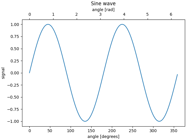
有时我们希望在绘图上有一个次坐标轴,例如在同一绘图上将弧度转换为度数.我们可以通过创建一个子坐标轴来实现这一点,该子坐标轴只有一个轴通过 axes.Axes.secondary_xaxis 和 axes.Axes.secondary_yaxis 可见.这个次坐标轴可以通过在函数的关键字参数中提供正向和反向转换函数的元组,来具有与主轴不同的刻度:

import datetime

import matplotlib.pyplot as plt
import numpy as np

import matplotlib.dates as mdates

fig, ax = plt.subplots(layout='constrained')
x = np.arange(0, 360, 1)
y = np.sin(2 * x * np.pi / 180)
ax.plot(x, y)
ax.set_xlabel('angle [degrees]')
ax.set_ylabel('signal')
ax.set_title('Sine wave')


def deg2rad(x):
    return x * np.pi / 180


def rad2deg(x):
    return x * 180 / np.pi


secax = ax.secondary_xaxis('top', functions=(deg2rad, rad2deg))
secax.set_xlabel('angle [rad]')
plt.show()

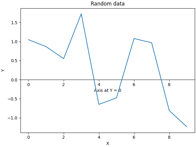
默认情况下,次坐标轴绘制在 Axes 坐标空间中.我们还可以提供一个自定义变换,将其放置在不同的坐标空间中.这里我们将轴放置在数据坐标中的 Y = 0 处.

fig, ax = plt.subplots(layout='constrained')
x = np.arange(0, 10)
np.random.seed(19680801)
y = np.random.randn(len(x))
ax.plot(x, y)
ax.set_xlabel('X')
ax.set_ylabel('Y')
ax.set_title('Random data')

# Pass ax.transData as a transform to place the axis relative to our data
secax = ax.secondary_xaxis(0, transform=ax.transData)
secax.set_xlabel('Axis at Y = 0')
plt.show()

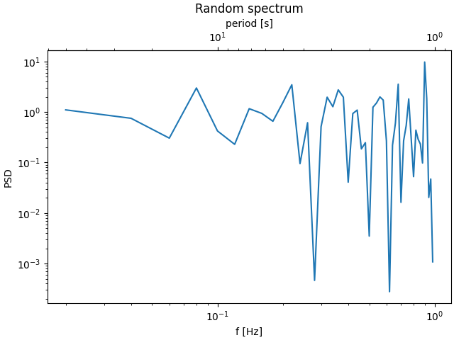
这是一个在对数刻度上从波数转换为波长的例子.

备注

在这种情况下,父级的 xscale 是对数的,因此子级也被设置为对数.

fig, ax = plt.subplots(layout='constrained')
x = np.arange(0.02, 1, 0.02)
np.random.seed(19680801)
y = np.random.randn(len(x)) ** 2
ax.loglog(x, y)
ax.set_xlabel('f [Hz]')
ax.set_ylabel('PSD')
ax.set_title('Random spectrum')


def one_over(x):
    """Vectorized 1/x, treating x==0 manually"""
    x = np.array(x, float)
    near_zero = np.isclose(x, 0)
    x[near_zero] = np.inf
    x[~near_zero] = 1 / x[~near_zero]
    return x


# the function "1/x" is its own inverse
inverse = one_over


secax = ax.secondary_xaxis('top', functions=(one_over, inverse))
secax.set_xlabel('period [s]')
plt.show()

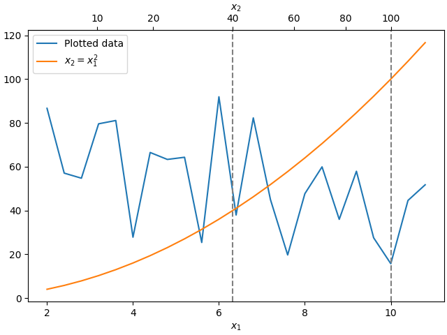
有时我们希望在一个从数据中临时派生的变换中关联轴,并且是根据经验得出的.或者,一个轴可能是另一个轴的复杂非线性函数.在这些情况下,我们可以将正向和反向变换函数设置为从一组自变量到另一组自变量的线性插值.

备注

为了正确处理数据边距,映射函数(本例中为 forward 和 inverse )需要定义在标称绘图限制之外.可以通过将插值扩展到绘制值之外(左右两侧)来强制执行此条件,请参见下面的 x1n 和 x2n .

fig, ax = plt.subplots(layout='constrained')
x1_vals = np.arange(2, 11, 0.4)
# second independent variable is a nonlinear function of the other.
x2_vals = x1_vals ** 2
ydata = 50.0 + 20 * np.random.randn(len(x1_vals))
ax.plot(x1_vals, ydata, label='Plotted data')
ax.plot(x1_vals, x2_vals, label=r'$x_2 = x_1^2$')
ax.set_xlabel(r'$x_1$')
ax.legend()

# the forward and inverse functions must be defined on the complete visible axis range
x1n = np.linspace(0, 20, 201)
x2n = x1n**2


def forward(x):
    return np.interp(x, x1n, x2n)


def inverse(x):
    return np.interp(x, x2n, x1n)

# use axvline to prove that the derived secondary axis is correctly plotted
ax.axvline(np.sqrt(40), color="grey", ls="--")
ax.axvline(10, color="grey", ls="--")
secax = ax.secondary_xaxis('top', functions=(forward, inverse))
secax.set_xticks([10, 20, 40, 60, 80, 100])
secax.set_xlabel(r'$x_2$')

plt.show()

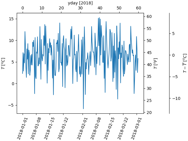
最后一个例子是将 np.datetime64 转换为 x 轴上的 yearday,并将 y 轴上的摄氏度转换为华氏度.请注意添加了第三个 y 轴,并且可以使用浮点数作为位置参数放置它

dates = [datetime.datetime(2018, 1, 1) + datetime.timedelta(hours=k * 6)
         for k in range(240)]
temperature = np.random.randn(len(dates)) * 4 + 6.7
fig, ax = plt.subplots(layout='constrained')

ax.plot(dates, temperature)
ax.set_ylabel(r'$T\ [^oC]$')
ax.xaxis.set_tick_params(rotation=70)


def date2yday(x):
    """Convert matplotlib datenum to days since 2018-01-01."""
    y = x - mdates.date2num(datetime.datetime(2018, 1, 1))
    return y


def yday2date(x):
    """Return a matplotlib datenum for *x* days after 2018-01-01."""
    y = x + mdates.date2num(datetime.datetime(2018, 1, 1))
    return y


secax_x = ax.secondary_xaxis('top', functions=(date2yday, yday2date))
secax_x.set_xlabel('yday [2018]')


def celsius_to_fahrenheit(x):
    return x * 1.8 + 32


def fahrenheit_to_celsius(x):
    return (x - 32) / 1.8


secax_y = ax.secondary_yaxis(
    'right', functions=(celsius_to_fahrenheit, fahrenheit_to_celsius))
secax_y.set_ylabel(r'$T\ [^oF]$')


def celsius_to_anomaly(x):
    return (x - np.mean(temperature))


def anomaly_to_celsius(x):
    return (x + np.mean(temperature))


# use of a float for the position:
secax_y2 = ax.secondary_yaxis(
    1.2, functions=(celsius_to_anomaly, anomaly_to_celsius))
secax_y2.set_ylabel(r'$T - \overline{T}\ [^oC]$')


plt.show()

参考

以下函数,方法,类和模块的用法在本例中显示:

• matplotlib.axes.Axes.secondary_xaxis

• matplotlib.axes.Axes.secondary_yaxis

标签:component: axis plot-type: line level: beginner