pcolormesh

axes.Axes.pcolormesh 允许你生成 2D 图像风格的绘图.请注意,它比类似的 pcolor 更快.

import matplotlib.pyplot as plt
import numpy as np

from matplotlib.colors import BoundaryNorm
from matplotlib.ticker import MaxNLocator

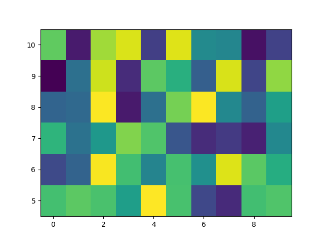
基本 pcolormesh

我们通常通过定义四边形的边缘和四边形的值来指定 pcolormesh.请注意,这里的 x 和 y 在各自的维度上都比 Z 多一个元素.

np.random.seed(19680801)
Z = np.random.rand(6, 10)
x = np.arange(-0.5, 10, 1)  # len = 11
y = np.arange(4.5, 11, 1)  # len = 7

fig, ax = plt.subplots()
ax.pcolormesh(x, y, Z)

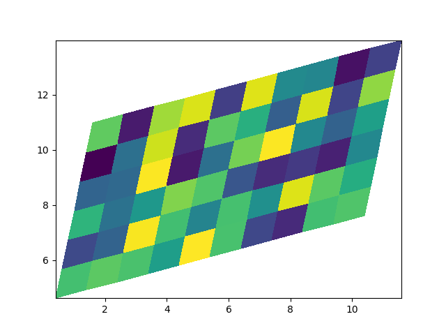
非直线 pcolormesh

请注意,我们也可以为 X 和 Y 指定矩阵,并拥有非直线的四边形.

x = np.arange(-0.5, 10, 1)  # len = 11
y = np.arange(4.5, 11, 1)  # len = 7
X, Y = np.meshgrid(x, y)
X = X + 0.2 * Y  # tilt the coordinates.
Y = Y + 0.3 * X

fig, ax = plt.subplots()
ax.pcolormesh(X, Y, Z)

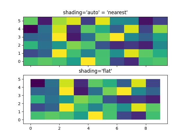
居中坐标

通常,用户希望传递与 Z 大小相同的 X 和 Y 到 axes.Axes.pcolormesh .如果传递了 shading='auto' ( rcParams["pcolor.shading"] (default: 'auto') 设置的默认值),也允许这样做.在 Matplotlib 3.3 之前, shading='flat' 会删除 Z 的最后一列和最后一行,但现在会报错. 如果这确实是你想要的,那么只需手动删除 Z 的最后一行和最后一列:

x = np.arange(10)  # len = 10
y = np.arange(6)  # len = 6
X, Y = np.meshgrid(x, y)

fig, axs = plt.subplots(2, 1, sharex=True, sharey=True)
axs[0].pcolormesh(X, Y, Z, vmin=np.min(Z), vmax=np.max(Z), shading='auto')
axs[0].set_title("shading='auto' = 'nearest'")
axs[1].pcolormesh(X, Y, Z[:-1, :-1], vmin=np.min(Z), vmax=np.max(Z),
                  shading='flat')
axs[1].set_title("shading='flat'")

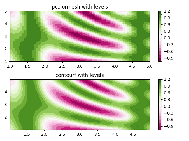
使用 Norms 创建 levels

展示了如何组合 Normalization 和 Colormap 实例,以类似于 contour/contourf 的 levels 关键字参数的方式,在 axes.Axes.pcolor , axes.Axes.pcolormesh 和 axes.Axes.imshow 类型的绘图中绘制"levels".

# make these smaller to increase the resolution
dx, dy = 0.05, 0.05

# generate 2 2d grids for the x & y bounds
y, x = np.mgrid[slice(1, 5 + dy, dy),
                slice(1, 5 + dx, dx)]

z = np.sin(x)**10 + np.cos(10 + y*x) * np.cos(x)

# x and y are bounds, so z should be the value *inside* those bounds.
# Therefore, remove the last value from the z array.
z = z[:-1, :-1]
levels = MaxNLocator(nbins=15).tick_values(z.min(), z.max())


# pick the desired colormap, sensible levels, and define a normalization
# instance which takes data values and translates those into levels.
cmap = plt.colormaps['PiYG']
norm = BoundaryNorm(levels, ncolors=cmap.N, clip=True)

fig, (ax0, ax1) = plt.subplots(nrows=2)

im = ax0.pcolormesh(x, y, z, cmap=cmap, norm=norm)
fig.colorbar(im, ax=ax0)
ax0.set_title('pcolormesh with levels')


# contours are *point* based plots, so convert our bound into point
# centers
cf = ax1.contourf(x[:-1, :-1] + dx/2.,
                  y[:-1, :-1] + dy/2., z, levels=levels,
                  cmap=cmap)
fig.colorbar(cf, ax=ax1)
ax1.set_title('contourf with levels')

# adjust spacing between subplots so `ax1` title and `ax0` tick labels
# don't overlap
fig.tight_layout()

plt.show()

参考

以下函数,方法,类和模块的用法在本例中显示:

• matplotlib.axes.Axes.pcolormesh / matplotlib.pyplot.pcolormesh

• matplotlib.axes.Axes.contourf / matplotlib.pyplot.contourf

• matplotlib.figure.Figure.colorbar / matplotlib.pyplot.colorbar

• matplotlib.colors.BoundaryNorm

• matplotlib.ticker.MaxNLocator