Asinh 演示

scale.AsinhScale 轴缩放的图示,它使用变换

\[a \rightarrow a_0 \sinh^{-1} (a / a_0)\]

对于接近零的坐标值(即远小于"线性宽度" \(a_0\) ),这使得值基本保持不变:

\[a \rightarrow a + \mathcal{O}(a^3)\]

但对于更大的值(即 \(|a| \gg a_0\) ),这渐近地为

\[a \rightarrow a_0 \, \mathrm{sgn}(a) \ln |a| + \mathcal{O}(1)\]

与 symlog 缩放一样,这允许绘制覆盖非常宽的动态范围(包括正值和负值)的量.但是, symlog 涉及在其梯度中具有不连续性的变换,因为它由单独的线性和对数变换构建. asinh 缩放使用的变换对于所有(有限)值都是平滑的,这在数学上更简洁,并减少了与绘图的线性和对数区域之间的突然过渡相关的视觉伪影.

备注

scale.AsinhScale 是实验性的,API 可能会更改.

请参见 AsinhScale , SymmetricalLogScale .

import matplotlib.pyplot as plt
import numpy as np

# Prepare sample values for variations on y=x graph:
x = np.linspace(-3, 6, 500)

比较样本 y=x 图上的 "symlog" 和 "asinh" 行为,其中 "symlog" 在 y=2 附近存在不连续的梯度:

fig1 = plt.figure()
ax0, ax1 = fig1.subplots(1, 2, sharex=True)

ax0.plot(x, x)
ax0.set_yscale('symlog')
ax0.grid()
ax0.set_title('symlog')

ax1.plot(x, x)
ax1.set_yscale('asinh')
ax1.grid()
ax1.set_title('asinh')

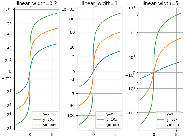
比较具有不同比例参数 "linear_width" 的 "asinh" 图:

fig2 = plt.figure(layout='constrained')
axs = fig2.subplots(1, 3, sharex=True)
for ax, (a0, base) in zip(axs, ((0.2, 2), (1.0, 0), (5.0, 10))):
    ax.set_title(f'linear_width={a0:.3g}')
    ax.plot(x, x, label='y=x')
    ax.plot(x, 10*x, label='y=10x')
    ax.plot(x, 100*x, label='y=100x')
    ax.set_yscale('asinh', linear_width=a0, base=base)
    ax.grid()
    ax.legend(loc='best', fontsize='small')

比较 2D 柯西分布随机数上的 "symlog" 和 "asinh" 缩放,其中可能能够看到在 y=2 附近的由于 "symlog" 中的梯度不连续性导致的更微妙的伪影:

fig3 = plt.figure()
ax = fig3.subplots(1, 1)
r = 3 * np.tan(np.random.uniform(-np.pi / 2.02, np.pi / 2.02,
                                 size=(5000,)))
th = np.random.uniform(0, 2*np.pi, size=r.shape)

ax.scatter(r * np.cos(th), r * np.sin(th), s=4, alpha=0.5)
ax.set_xscale('asinh')
ax.set_yscale('symlog')
ax.set_xlabel('asinh')
ax.set_ylabel('symlog')
ax.set_title('2D Cauchy random deviates')
ax.set_xlim(-50, 50)
ax.set_ylim(-50, 50)
ax.grid()

plt.show()

参考

• matplotlib.scale.AsinhScale

• matplotlib.ticker.AsinhLocator

• matplotlib.scale.SymmetricalLogScale