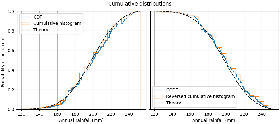
累积分布

此示例展示了如何绘制样本的经验累积分布函数 (ECDF).我们还展示了理论 CDF.

在工程学中,ECDF 有时被称为"非超越"曲线:给定 x 值的 y 值给出了样本中的观察值低于该 x 值的概率.例如,x 轴上 220 的值对应于 y 轴上大约 0.80,因此样本中的观察值不超过 220 的概率为 80%.相反,经验互补累积分布函数(ECCDF,或"超越"曲线)显示了样本中的观察值高于值 x 的概率 y.

绘制 ECDF 的直接方法是 Axes.ecdf .传递 complementary=True 会产生 ECCDF.

或者,可以使用 ax.hist(data, density=True, cumulative=True) 首先对数据进行分箱,就像绘制直方图一样,然后计算并绘制每个箱中条目的频率的累积和.在这里,要绘制 ECCDF,请传递 cumulative=-1 .请注意,此方法会导致 E(C)CDF 的近似值,而 Axes.ecdf 是精确的.

import matplotlib.pyplot as plt
import numpy as np

np.random.seed(19680801)

mu = 200
sigma = 25
n_bins = 25
data = np.random.normal(mu, sigma, size=100)

fig = plt.figure(figsize=(9, 4), layout="constrained")
axs = fig.subplots(1, 2, sharex=True, sharey=True)

# Cumulative distributions.
axs[0].ecdf(data, label="CDF")
n, bins, patches = axs[0].hist(data, n_bins, density=True, histtype="step",
                               cumulative=True, label="Cumulative histogram")
x = np.linspace(data.min(), data.max())
y = ((1 / (np.sqrt(2 * np.pi) * sigma)) *
     np.exp(-0.5 * (1 / sigma * (x - mu))**2))
y = y.cumsum()
y /= y[-1]
axs[0].plot(x, y, "k--", linewidth=1.5, label="Theory")

# Complementary cumulative distributions.
axs[1].ecdf(data, complementary=True, label="CCDF")
axs[1].hist(data, bins=bins, density=True, histtype="step", cumulative=-1,
            label="Reversed cumulative histogram")
axs[1].plot(x, 1 - y, "k--", linewidth=1.5, label="Theory")

# Label the figure.
fig.suptitle("Cumulative distributions")
for ax in axs:
    ax.grid(True)
    ax.legend()
    ax.set_xlabel("Annual rainfall (mm)")
    ax.set_ylabel("Probability of occurrence")
    ax.label_outer()

plt.show()

Tags: plot-type: ecdf plot-type: histogram domain: statistics

参考

以下函数,方法,类和模块的用法在本例中显示:

• matplotlib.axes.Axes.hist / matplotlib.pyplot.hist

• matplotlib.axes.Axes.ecdf / matplotlib.pyplot.ecdf