绘制二维数据集的置信椭圆

此示例展示了如何使用二维数据集的皮尔逊相关系数绘制其置信椭圆.

获取正确几何形状的方法在此处进行了解释和证明:

https://carstenschelp.github.io/2018/09/14/Plot_Confidence_Ellipse_001.html

该方法避免了使用迭代特征分解算法,并且利用了归一化协方差矩阵(由皮尔逊相关系数和1组成)特别容易处理这一事实.

import matplotlib.pyplot as plt
import numpy as np

from matplotlib.patches import Ellipse
import matplotlib.transforms as transforms

绘图函数本身

此函数绘制给定类数组变量 x 和 y 的协方差的置信椭圆. 椭圆被绘制到给定的 Axes 对象 ax 中.

椭圆的半径可以通过 n_std 来控制,它是标准偏差的数量. 默认值为 3,如果数据像这些例子中一样呈正态分布,则椭圆会包围 98.9% 的点(1-D 中的 3 个标准差包含 99.7% 的数据,这相当于 2-D 中的 98.9% 的数据).

def confidence_ellipse(x, y, ax, n_std=3.0, facecolor='none', **kwargs):
    """
    Create a plot of the covariance confidence ellipse of *x* and *y*.

    Parameters
    ----------
    x, y : array-like, shape (n, )
        Input data.

    ax : matplotlib.axes.Axes
        The Axes object to draw the ellipse into.

    n_std : float
        The number of standard deviations to determine the ellipse's radiuses.

    **kwargs
        Forwarded to `~matplotlib.patches.Ellipse`

    Returns
    -------
    matplotlib.patches.Ellipse
    """
    if x.size != y.size:
        raise ValueError("x and y must be the same size")

    cov = np.cov(x, y)
    pearson = cov[0, 1]/np.sqrt(cov[0, 0] * cov[1, 1])
    # Using a special case to obtain the eigenvalues of this
    # two-dimensional dataset.
    ell_radius_x = np.sqrt(1 + pearson)
    ell_radius_y = np.sqrt(1 - pearson)
    ellipse = Ellipse((0, 0), width=ell_radius_x * 2, height=ell_radius_y * 2,
                      facecolor=facecolor, **kwargs)

    # Calculating the standard deviation of x from
    # the squareroot of the variance and multiplying
    # with the given number of standard deviations.
    scale_x = np.sqrt(cov[0, 0]) * n_std
    mean_x = np.mean(x)

    # calculating the standard deviation of y ...
    scale_y = np.sqrt(cov[1, 1]) * n_std
    mean_y = np.mean(y)

    transf = transforms.Affine2D() \
        .rotate_deg(45) \
        .scale(scale_x, scale_y) \
        .translate(mean_x, mean_y)

    ellipse.set_transform(transf + ax.transData)
    return ax.add_patch(ellipse)

用于创建相关数据集的辅助函数

创建具有指定的二维均值 (mu) 和维度 (scale) 的随机二维数据集. 相关性可以通过参数"dependency"(一个 2x2 矩阵)来控制.

def get_correlated_dataset(n, dependency, mu, scale):
    latent = np.random.randn(n, 2)
    dependent = latent.dot(dependency)
    scaled = dependent * scale
    scaled_with_offset = scaled + mu
    # return x and y of the new, correlated dataset
    return scaled_with_offset[:, 0], scaled_with_offset[:, 1]

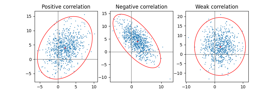
正相关,负相关和弱相关

请注意,弱相关(右图)的形状是椭圆,而不是圆形,因为 x 和 y 的比例不同. 然而,x 和 y 不相关的事实通过椭圆的轴与坐标系的 x 轴和 y 轴对齐来表示.

np.random.seed(0)

PARAMETERS = {
    'Positive correlation': [[0.85, 0.35],
                             [0.15, -0.65]],
    'Negative correlation': [[0.9, -0.4],
                             [0.1, -0.6]],
    'Weak correlation': [[1, 0],
                         [0, 1]],
}

mu = 2, 4
scale = 3, 5

fig, axs = plt.subplots(1, 3, figsize=(9, 3))
for ax, (title, dependency) in zip(axs, PARAMETERS.items()):
    x, y = get_correlated_dataset(800, dependency, mu, scale)
    ax.scatter(x, y, s=0.5)

    ax.axvline(c='grey', lw=1)
    ax.axhline(c='grey', lw=1)

    confidence_ellipse(x, y, ax, edgecolor='red')

    ax.scatter(mu[0], mu[1], c='red', s=3)
    ax.set_title(title)

plt.show()

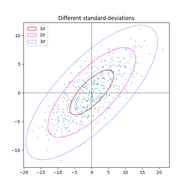
不同的标准差数量

n_std = 3(蓝色),2(紫色)和 1(红色)的绘图

fig, ax_nstd = plt.subplots(figsize=(6, 6))

dependency_nstd = [[0.8, 0.75],
                   [-0.2, 0.35]]
mu = 0, 0
scale = 8, 5

ax_nstd.axvline(c='grey', lw=1)
ax_nstd.axhline(c='grey', lw=1)

x, y = get_correlated_dataset(500, dependency_nstd, mu, scale)
ax_nstd.scatter(x, y, s=0.5)

confidence_ellipse(x, y, ax_nstd, n_std=1,
                   label=r'$1\sigma$', edgecolor='firebrick')
confidence_ellipse(x, y, ax_nstd, n_std=2,
                   label=r'$2\sigma$', edgecolor='fuchsia', linestyle='--')
confidence_ellipse(x, y, ax_nstd, n_std=3,
                   label=r'$3\sigma$', edgecolor='blue', linestyle=':')

ax_nstd.scatter(mu[0], mu[1], c='red', s=3)
ax_nstd.set_title('Different standard deviations')
ax_nstd.legend()
plt.show()

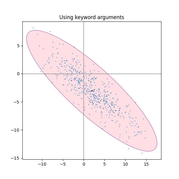
使用关键字参数

使用为 matplotlib.patches.Patch 指定的关键字参数,以便以不同的方式呈现椭圆.

fig, ax_kwargs = plt.subplots(figsize=(6, 6))
dependency_kwargs = [[-0.8, 0.5],
                     [-0.2, 0.5]]
mu = 2, -3
scale = 6, 5

ax_kwargs.axvline(c='grey', lw=1)
ax_kwargs.axhline(c='grey', lw=1)

x, y = get_correlated_dataset(500, dependency_kwargs, mu, scale)
# Plot the ellipse with zorder=0 in order to demonstrate
# its transparency (caused by the use of alpha).
confidence_ellipse(x, y, ax_kwargs,
                   alpha=0.5, facecolor='pink', edgecolor='purple', zorder=0)

ax_kwargs.scatter(x, y, s=0.5)
ax_kwargs.scatter(mu[0], mu[1], c='red', s=3)
ax_kwargs.set_title('Using keyword arguments')

fig.subplots_adjust(hspace=0.25)
plt.show()

Tags: plot-type: speciality plot-type: scatter component: ellipse component: patch domain: statistics

参考

以下函数,方法,类和模块的用法在本例中显示:

• matplotlib.transforms.Affine2D

• matplotlib.patches.Ellipse