备注
Go to the end 下载完整的示例代码.
直方图箱,密度和权重#
Axes.hist 方法可以灵活地以几种不同的方式创建直方图,这既灵活又有帮助,但也可能导致混淆.特别是,您可以:
根据需要对数据进行分箱,可以使用自动选择的箱数,也可以使用固定的箱边缘,
对直方图进行归一化,使其积分为 1,
并为数据点分配权重,以便每个数据点以不同的方式影响其箱中的计数.
Matplotlib 的 hist 方法调用 numpy.histogram 并绘制结果,因此用户应参考 numpy 文档以获取明确的指南.
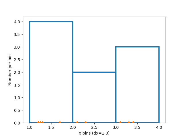
直方图是通过定义箱边缘,获取值数据集并将其排序到箱中,以及计算或求和每个箱中的数据量来创建的.在这个简单的例子中,9 个介于 1 和 4 之间的数字被排序到 3 个箱中:
import matplotlib.pyplot as plt
import numpy as np

rng = np.random.default_rng(19680801)

xdata = np.array([1.2, 2.3, 3.3, 3.1, 1.7, 3.4, 2.1, 1.25, 1.3])
xbins = np.array([1, 2, 3, 4])

# changing the style of the histogram bars just to make it
# very clear where the boundaries of the bins are:
style = {'facecolor': 'none', 'edgecolor': 'C0', 'linewidth': 3}

fig, ax = plt.subplots()
ax.hist(xdata, bins=xbins, **style)

# plot the xdata locations on the x axis:
ax.plot(xdata, 0*xdata, 'd')
ax.set_ylabel('Number per bin')
ax.set_xlabel('x bins (dx=1.0)')
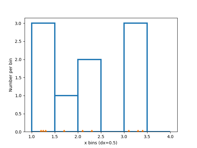
修改箱#
更改箱的大小会改变这个稀疏直方图的形状,因此最好根据您的数据谨慎选择箱.在这里,我们将箱的宽度缩小了一半.
xbins = np.arange(1, 4.5, 0.5)

fig, ax = plt.subplots()
ax.hist(xdata, bins=xbins, **style)
ax.plot(xdata, 0*xdata, 'd')
ax.set_ylabel('Number per bin')
ax.set_xlabel('x bins (dx=0.5)')
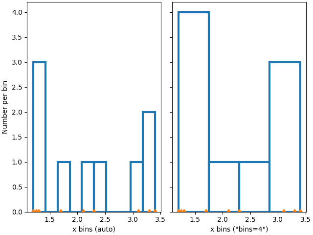
我们还可以让 numpy(通过 Matplotlib)自动选择箱,或者指定要自动选择的箱的数量:
fig, ax = plt.subplot_mosaic([['auto', 'n4']],
                             sharex=True, sharey=True, layout='constrained')

ax['auto'].hist(xdata, **style)
ax['auto'].plot(xdata, 0*xdata, 'd')
ax['auto'].set_ylabel('Number per bin')
ax['auto'].set_xlabel('x bins (auto)')

ax['n4'].hist(xdata, bins=4, **style)
ax['n4'].plot(xdata, 0*xdata, 'd')
ax['n4'].set_xlabel('x bins ("bins=4")')
归一化直方图:密度和权重#
每个箱的计数是直方图中每个条的默认长度.但是,我们也可以使用 density 参数将条的长度归一化为概率密度函数:
fig, ax = plt.subplots()
ax.hist(xdata, bins=xbins, density=True, **style)
ax.set_ylabel('Probability density [$V^{-1}$])')
ax.set_xlabel('x bins (dx=0.5 $V$)')
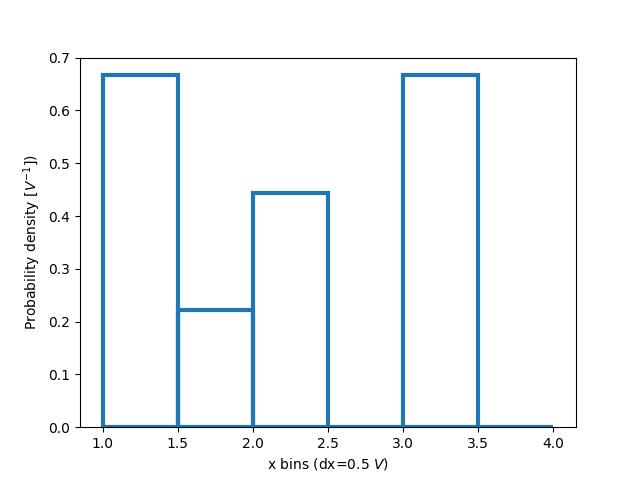
当仅探索数据时,这种归一化可能有点难以解释.附加到每个条的值除以数据点的总数和箱的宽度,因此当在整个数据范围内积分时,值 _积分_ 为 1.例如:
density = counts / (sum(counts) * np.diff(bins))
np.sum(density * np.diff(bins)) == 1
这种归一化是统计学中 probability density functions 的定义方式.如果 \(X\) 是 \(x\) 上的随机变量,那么 \(f_X\) 是概率密度函数,如果 \(P[a<X<b] = \int_a^b f_X dx\) .如果 x 的单位是伏特,那么 \(f_X\) 的单位是 \(V^{-1}\) 或每次电压变化的概率.
当我们从已知分布中抽取并尝试与理论进行比较时,这种归一化的有用性会更清晰一些.因此,从 normal distribution 中选择 1000 个点,并计算已知的概率密度函数:
xdata = rng.normal(size=1000)
xpdf = np.arange(-4, 4, 0.1)
pdf = 1 / (np.sqrt(2 * np.pi)) * np.exp(-xpdf**2 / 2)
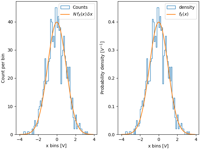
如果我们不使用 density=True ,我们需要按数据的长度和箱的宽度来缩放预期的概率分布函数:
fig, ax = plt.subplot_mosaic([['False', 'True']], layout='constrained')
dx = 0.1
xbins = np.arange(-4, 4, dx)
ax['False'].hist(xdata, bins=xbins, density=False, histtype='step', label='Counts')

# scale and plot the expected pdf:
ax['False'].plot(xpdf, pdf * len(xdata) * dx, label=r'$N\,f_X(x)\,\delta x$')
ax['False'].set_ylabel('Count per bin')
ax['False'].set_xlabel('x bins [V]')
ax['False'].legend()

ax['True'].hist(xdata, bins=xbins, density=True, histtype='step', label='density')
ax['True'].plot(xpdf, pdf, label='$f_X(x)$')
ax['True'].set_ylabel('Probability density [$V^{-1}$]')
ax['True'].set_xlabel('x bins [$V$]')
ax['True'].legend()
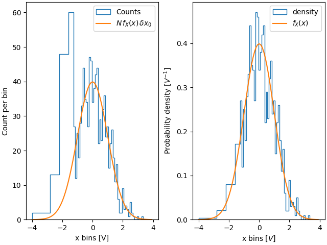
因此,使用密度的优点之一是直方图的形状和幅度不依赖于箱的大小.考虑一个箱宽度不同的极端情况.在此示例中,低于 x=-1.25 的箱比其余箱宽六倍.通过按密度归一化,我们保留了分布的形状,而如果我们不这样做,那么更宽的箱的计数将远高于更窄的箱:
fig, ax = plt.subplot_mosaic([['False', 'True']], layout='constrained')
dx = 0.1
xbins = np.hstack([np.arange(-4, -1.25, 6*dx), np.arange(-1.25, 4, dx)])
ax['False'].hist(xdata, bins=xbins, density=False, histtype='step', label='Counts')
ax['False'].plot(xpdf, pdf * len(xdata) * dx, label=r'$N\,f_X(x)\,\delta x_0$')
ax['False'].set_ylabel('Count per bin')
ax['False'].set_xlabel('x bins [V]')
ax['False'].legend()

ax['True'].hist(xdata, bins=xbins, density=True, histtype='step', label='density')
ax['True'].plot(xpdf, pdf, label='$f_X(x)$')
ax['True'].set_ylabel('Probability density [$V^{-1}$]')
ax['True'].set_xlabel('x bins [$V$]')
ax['True'].legend()
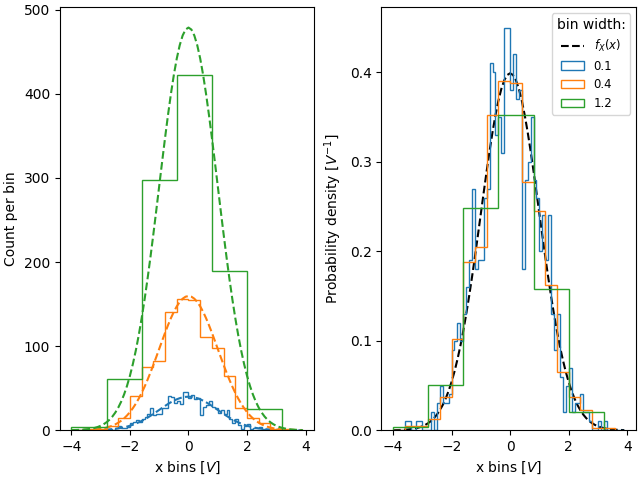
类似地,如果我们想要比较具有不同 bin 宽度的直方图,我们可以使用 density=True :
fig, ax = plt.subplot_mosaic([['False', 'True']], layout='constrained')

# expected PDF
ax['True'].plot(xpdf, pdf, '--', label='$f_X(x)$', color='k')

for nn, dx in enumerate([0.1, 0.4, 1.2]):
    xbins = np.arange(-4, 4, dx)
    # expected histogram:
    ax['False'].plot(xpdf, pdf*1000*dx, '--', color=f'C{nn}')
    ax['False'].hist(xdata, bins=xbins, density=False, histtype='step')

    ax['True'].hist(xdata, bins=xbins, density=True, histtype='step', label=dx)

# Labels:
ax['False'].set_xlabel('x bins [$V$]')
ax['False'].set_ylabel('Count per bin')
ax['True'].set_ylabel('Probability density [$V^{-1}$]')
ax['True'].set_xlabel('x bins [$V$]')
ax['True'].legend(fontsize='small', title='bin width:')
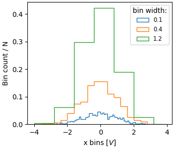
有时人们想要归一化,使得计数之和为 1.这类似于离散变量的 probability mass function ,其中所有值的概率之和等于 1.使用 hist ,如果我们将权重设置为 1/N,我们可以获得这种归一化.请注意,此标准化直方图的幅度仍然取决于 bin 的宽度和/或数量:
fig, ax = plt.subplots(layout='constrained', figsize=(3.5, 3))

for nn, dx in enumerate([0.1, 0.4, 1.2]):
    xbins = np.arange(-4, 4, dx)
    ax.hist(xdata, bins=xbins, weights=1/len(xdata) * np.ones(len(xdata)),
                   histtype='step', label=f'{dx}')
ax.set_xlabel('x bins [$V$]')
ax.set_ylabel('Bin count / N')
ax.legend(fontsize='small', title='bin width:')
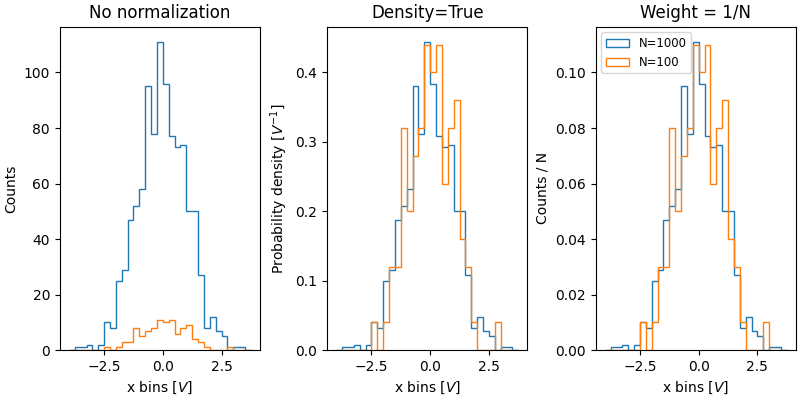
规范化直方图的价值在于比较具有不同大小人口的两个分布.在这里,我们将具有 1000 个成员的 xdata 分布与具有 100 个成员的 xdata2 分布进行比较.
xdata2 = rng.normal(size=100)

fig, ax = plt.subplot_mosaic([['no_norm', 'density', 'weight']],
                             layout='constrained', figsize=(8, 4))

xbins = np.arange(-4, 4, 0.25)

ax['no_norm'].hist(xdata, bins=xbins, histtype='step')
ax['no_norm'].hist(xdata2, bins=xbins, histtype='step')
ax['no_norm'].set_ylabel('Counts')
ax['no_norm'].set_xlabel('x bins [$V$]')
ax['no_norm'].set_title('No normalization')

ax['density'].hist(xdata, bins=xbins, histtype='step', density=True)
ax['density'].hist(xdata2, bins=xbins, histtype='step', density=True)
ax['density'].set_ylabel('Probability density [$V^{-1}$]')
ax['density'].set_title('Density=True')
ax['density'].set_xlabel('x bins [$V$]')

ax['weight'].hist(xdata, bins=xbins, histtype='step',
                  weights=1 / len(xdata) * np.ones(len(xdata)),
                  label='N=1000')
ax['weight'].hist(xdata2, bins=xbins, histtype='step',
                  weights=1 / len(xdata2) * np.ones(len(xdata2)),
                  label='N=100')
ax['weight'].set_xlabel('x bins [$V$]')
ax['weight'].set_ylabel('Counts / N')
ax['weight'].legend(fontsize='small')
ax['weight'].set_title('Weight = 1/N')

plt.show()
参考
以下函数,方法,类和模块的用法在本例中显示:
matplotlib.axes.Axes.hist/matplotlib.pyplot.histmatplotlib.axes.Axes.set_titlematplotlib.axes.Axes.set_xlabelmatplotlib.axes.Axes.set_ylabelmatplotlib.axes.Axes.legend
脚本的总运行时间:(0 分钟 4.193 秒)