从颜色列表创建 colormap

有关创建和操作 colormap 的更多详细信息,请参阅 在 Matplotlib 中创建颜色映射 .

从颜色列表创建 colormap 可以使用 LinearSegmentedColormap.from_list 方法完成.您必须传递一个 RGB 元组列表,该列表定义了从 0 到 1 的颜色混合.

创建自定义 colormap

也可以为 colormap 创建自定义映射.这可以通过创建一个字典来实现,该字典指定 RGB 通道如何从 cmap 的一端变化到另一端.

例如:假设您希望红色在下半部分从 0 增加到 1,绿色在中间一半做同样的事情,蓝色在上半部分做同样的事情.那么您将使用:

cdict = {
    'red': (
        (0.0,  0.0, 0.0),
        (0.5,  1.0, 1.0),
        (1.0,  1.0, 1.0),
    ),
    'green': (
        (0.0,  0.0, 0.0),
        (0.25, 0.0, 0.0),
        (0.75, 1.0, 1.0),
        (1.0,  1.0, 1.0),
    ),
    'blue': (
        (0.0,  0.0, 0.0),
        (0.5,  0.0, 0.0),
        (1.0,  1.0, 1.0),
    )
}

如果像本例一样,r,g 和 b 分量中没有不连续性,那么这非常简单:上面每个元组的第二个和第三个元素是相同的--称之为"y ".第一个元素("x ")定义了 0 到 1 完整范围内的插值间隔,并且它必须跨越整个范围.换句话说, x 的值将 0 到 1 的范围划分为一组段,而 y 给出了每个段的端点颜色值.

现在考虑绿色, cdict['green'] 表示:

• 0 <= x <= 0.25, y 为零;没有绿色.

• 0.25 < x <= 0.75, y 从 0 线性变化到 1.

• 0.75 < x <= 1, y 保持在 1,全绿色.

如果存在不连续性,那么它会稍微复杂一些.将 cdict 条目中给定颜色的每一行中的 3 个元素标记为 (x, y0, y1) .然后,对于 x[i] 和 x[i+1] 之间的 x 值,颜色值在 y1[i] 和 y0[i+1] 之间插值.

回到一个 cookbook 示例:

cdict = {
    'red': (
        (0.0,  0.0, 0.0),
        (0.5,  1.0, 0.7),
        (1.0,  1.0, 1.0),
    ),
    'green': (
        (0.0,  0.0, 0.0),
        (0.5,  1.0, 0.0),
        (1.0,  1.0, 1.0),
    ),
    'blue': (
        (0.0,  0.0, 0.0),
        (0.5,  0.0, 0.0),
        (1.0,  1.0, 1.0),
    )
}

并查看 cdict['red'][1] ;因为 y0 != y1 ,它表示对于从 0 到 0.5 的 x ,红色从 0 增加到 1,但随后它跳下来,因此对于从 0.5 到 1 的 x ,红色从 0.7 增加到 1.当 x 从 0 到 0.5 时,绿色从 0 线性变化到 1,然后跳回到 0,并当 x 从 0.5 到 1 时线性变化回 1.:

row i:   x  y0  y1
               /
              /
row i+1: x  y0  y1

上面试图表明,对于 x 在 x[i] 到 x[i+1] 范围内,插值在 y1[i] 和 y0[i+1] 之间.因此,永远不会使用 y0[0] 和 y1[-1] .

import matplotlib.pyplot as plt
import numpy as np

import matplotlib as mpl
from matplotlib.colors import LinearSegmentedColormap

# Make some illustrative fake data:

x = np.arange(0, np.pi, 0.1)
y = np.arange(0, 2 * np.pi, 0.1)
X, Y = np.meshgrid(x, y)
Z = np.cos(X) * np.sin(Y) * 10

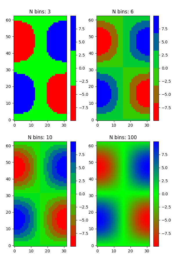
来自列表的 Colormap

colors = [(1, 0, 0), (0, 1, 0), (0, 0, 1)]  # R -> G -> B
n_bins = [3, 6, 10, 100]  # Discretizes the interpolation into bins
cmap_name = 'my_list'
fig, axs = plt.subplots(2, 2, figsize=(6, 9))
fig.subplots_adjust(left=0.02, bottom=0.06, right=0.95, top=0.94, wspace=0.05)
for n_bin, ax in zip(n_bins, axs.flat):
    # Create the colormap
    cmap = LinearSegmentedColormap.from_list(cmap_name, colors, N=n_bin)
    # Fewer bins will result in "coarser" colomap interpolation
    im = ax.imshow(Z, origin='lower', cmap=cmap)
    ax.set_title("N bins: %s" % n_bin)
    fig.colorbar(im, ax=ax)

自定义 colormap

cdict1 = {
    'red': (
        (0.0, 0.0, 0.0),
        (0.5, 0.0, 0.1),
        (1.0, 1.0, 1.0),
    ),
    'green': (
        (0.0, 0.0, 0.0),
        (1.0, 0.0, 0.0),
    ),
    'blue': (
        (0.0, 0.0, 1.0),
        (0.5, 0.1, 0.0),
        (1.0, 0.0, 0.0),
    )
}

cdict2 = {
    'red': (
        (0.0, 0.0, 0.0),
        (0.5, 0.0, 1.0),
        (1.0, 0.1, 1.0),
    ),
    'green': (
        (0.0, 0.0, 0.0),
        (1.0, 0.0, 0.0),
    ),
    'blue': (
        (0.0, 0.0, 0.1),
        (0.5, 1.0, 0.0),
        (1.0, 0.0, 0.0),
    )
}

cdict3 = {
    'red': (
        (0.0, 0.0, 0.0),
        (0.25, 0.0, 0.0),
        (0.5, 0.8, 1.0),
        (0.75, 1.0, 1.0),
        (1.0, 0.4, 1.0),
    ),
    'green': (
        (0.0, 0.0, 0.0),
        (0.25, 0.0, 0.0),
        (0.5, 0.9, 0.9),
        (0.75, 0.0, 0.0),
        (1.0, 0.0, 0.0),
    ),
    'blue': (
        (0.0, 0.0, 0.4),
        (0.25, 1.0, 1.0),
        (0.5, 1.0, 0.8),
        (0.75, 0.0, 0.0),
        (1.0, 0.0, 0.0),
    )
}

# Make a modified version of cdict3 with some transparency
# in the middle of the range.
cdict4 = {
    **cdict3,
    'alpha': (
        (0.0, 1.0, 1.0),
        # (0.25, 1.0, 1.0),
        (0.5, 0.3, 0.3),
        # (0.75, 1.0, 1.0),
        (1.0, 1.0, 1.0),
    ),
}

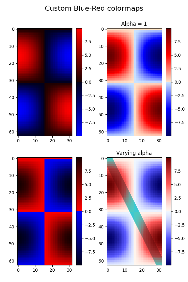
现在我们将使用这个例子来说明处理自定义 colormap 的 2 种方法.首先,最直接和显式的方法:

blue_red1 = LinearSegmentedColormap('BlueRed1', cdict1)

其次,显式创建映射并注册它.与第一种方法一样,此方法适用于任何类型的 Colormap,而不仅仅是 LinearSegmentedColormap:

mpl.colormaps.register(LinearSegmentedColormap('BlueRed2', cdict2))
mpl.colormaps.register(LinearSegmentedColormap('BlueRed3', cdict3))
mpl.colormaps.register(LinearSegmentedColormap('BlueRedAlpha', cdict4))

制作带有 4 个子图的图形:

fig, axs = plt.subplots(2, 2, figsize=(6, 9))
fig.subplots_adjust(left=0.02, bottom=0.06, right=0.95, top=0.94, wspace=0.05)

im1 = axs[0, 0].imshow(Z, cmap=blue_red1)
fig.colorbar(im1, ax=axs[0, 0])

im2 = axs[1, 0].imshow(Z, cmap='BlueRed2')
fig.colorbar(im2, ax=axs[1, 0])

# Now we will set the third cmap as the default.  One would
# not normally do this in the middle of a script like this;
# it is done here just to illustrate the method.

plt.rcParams['image.cmap'] = 'BlueRed3'

im3 = axs[0, 1].imshow(Z)
fig.colorbar(im3, ax=axs[0, 1])
axs[0, 1].set_title("Alpha = 1")

# Or as yet another variation, we can replace the rcParams
# specification *before* the imshow with the following *after*
# imshow.
# This sets the new default *and* sets the colormap of the last
# image-like item plotted via pyplot, if any.
#

# Draw a line with low zorder so it will be behind the image.
axs[1, 1].plot([0, 10 * np.pi], [0, 20 * np.pi], color='c', lw=20, zorder=-1)

im4 = axs[1, 1].imshow(Z)
fig.colorbar(im4, ax=axs[1, 1])

# Here it is: changing the colormap for the current image and its
# colorbar after they have been plotted.
im4.set_cmap('BlueRedAlpha')
axs[1, 1].set_title("Varying alpha")

fig.suptitle('Custom Blue-Red colormaps', fontsize=16)
fig.subplots_adjust(top=0.9)

plt.show()

参考

以下函数,方法,类和模块的用法在本例中显示:

• matplotlib.axes.Axes.imshow / matplotlib.pyplot.imshow

• matplotlib.figure.Figure.colorbar / matplotlib.pyplot.colorbar

• matplotlib.colors

• matplotlib.colors.LinearSegmentedColormap

• matplotlib.colors.LinearSegmentedColormap.from_list

• matplotlib.cm

• matplotlib.cm.ScalarMappable.set_cmap

• matplotlib.cm.ColormapRegistry.register

Tags: styling: colormap plot-type: imshow level: intermediate