备注
Go to the end 下载完整的示例代码.
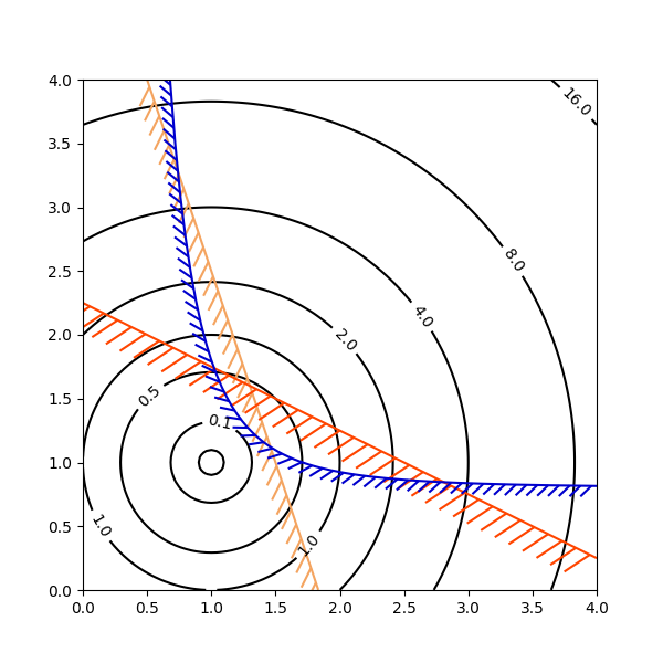
优化解决方案空间的等高线图#
在说明优化问题的解空间时,等高线绘图特别方便.不仅可以使用 axes.Axes.contour 来表示目标函数的地形,还可以使用它来生成约束函数的边界曲线.约束线可以用 TickedStroke 绘制,以区分约束边界的有效侧和无效侧.
matplotlib.axes.Axes.contour 生成的曲线在等高线的左侧具有较大的值.角度参数测量的是前进方向的零度,值向左增加.因此,当使用 TickedStroke 说明典型优化问题中的约束时,角度应设置在零到 180 度之间.
import matplotlib.pyplot as plt
import numpy as np

from matplotlib import patheffects

fig, ax = plt.subplots(figsize=(6, 6))

nx = 101
ny = 105

# Set up survey vectors
xvec = np.linspace(0.001, 4.0, nx)
yvec = np.linspace(0.001, 4.0, ny)

# Set up survey matrices.  Design disk loading and gear ratio.
x1, x2 = np.meshgrid(xvec, yvec)

# Evaluate some stuff to plot
obj = x1**2 + x2**2 - 2*x1 - 2*x2 + 2
g1 = -(3*x1 + x2 - 5.5)
g2 = -(x1 + 2*x2 - 4.5)
g3 = 0.8 + x1**-3 - x2

cntr = ax.contour(x1, x2, obj, [0.01, 0.1, 0.5, 1, 2, 4, 8, 16],
                  colors='black')
ax.clabel(cntr, fmt="%2.1f", use_clabeltext=True)

cg1 = ax.contour(x1, x2, g1, [0], colors='sandybrown')
cg1.set(path_effects=[patheffects.withTickedStroke(angle=135)])

cg2 = ax.contour(x1, x2, g2, [0], colors='orangered')
cg2.set(path_effects=[patheffects.withTickedStroke(angle=60, length=2)])

cg3 = ax.contour(x1, x2, g3, [0], colors='mediumblue')
cg3.set(path_effects=[patheffects.withTickedStroke(spacing=7)])

ax.set_xlim(0, 4)
ax.set_ylim(0, 4)

plt.show()