阶梯演示

此示例演示了如何使用 stairs 来绘制阶跃常数函数.一个常见的用例是直方图和类似直方图的数据可视化.

import matplotlib.pyplot as plt
import numpy as np

from matplotlib.patches import StepPatch

np.random.seed(0)
h, edges = np.histogram(np.random.normal(5, 3, 5000),
                        bins=np.linspace(0, 10, 20))

fig, axs = plt.subplots(3, 1, figsize=(7, 15))
axs[0].stairs(h, edges, label='Simple histogram')
axs[0].stairs(h, edges + 5, baseline=50, label='Modified baseline')
axs[0].stairs(h, edges + 10, baseline=None, label='No edges')
axs[0].set_title("Step Histograms")

axs[1].stairs(np.arange(1, 6, 1), fill=True,
              label='Filled histogram\nw/ automatic edges')
axs[1].stairs(np.arange(1, 6, 1)*0.3, np.arange(2, 8, 1),
              orientation='horizontal', hatch='//',
              label='Hatched histogram\nw/ horizontal orientation')
axs[1].set_title("Filled histogram")

patch = StepPatch(values=[1, 2, 3, 2, 1],
                  edges=range(1, 7),
                  label=('Patch derived underlying object\n'
                         'with default edge/facecolor behaviour'))
axs[2].add_patch(patch)
axs[2].set_xlim(0, 7)
axs[2].set_ylim(-1, 5)
axs[2].set_title("StepPatch artist")

for ax in axs:
    ax.legend()
plt.show()

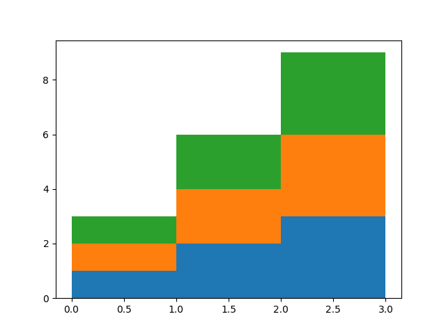
baseline 可以采用数组来允许堆叠直方图的绘制

A = [[0, 0, 0],
     [1, 2, 3],
     [2, 4, 6],
     [3, 6, 9]]

for i in range(len(A) - 1):
    plt.stairs(A[i+1], baseline=A[i], fill=True)

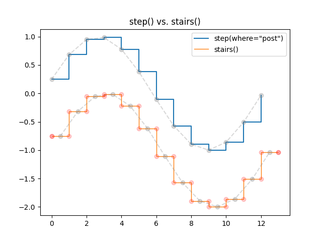
比较 pyplot.step 和 pyplot.stairs

pyplot.step 将步长位置定义为单个值.步长从这些参考值向左/向右/双向延伸,具体取决于参数 where.x 和 y 值的数量相同.

相反, pyplot.stairs 通过其边界 edges 定义步长位置,该位置比步长值长一个元素.

bins = np.arange(14)
centers = bins[:-1] + np.diff(bins) / 2
y = np.sin(centers / 2)

plt.step(bins[:-1], y, where='post', label='step(where="post")')
plt.plot(bins[:-1], y, 'o--', color='grey', alpha=0.3)

plt.stairs(y - 1, bins, baseline=None, label='stairs()')
plt.plot(centers, y - 1, 'o--', color='grey', alpha=0.3)
plt.plot(np.repeat(bins, 2), np.hstack([y[0], np.repeat(y, 2), y[-1]]) - 1,
         'o', color='red', alpha=0.2)

plt.legend()
plt.title('step() vs. stairs()')
plt.show()

参考

以下函数,方法,类和模块的用法在本例中显示:

• matplotlib.axes.Axes.stairs / matplotlib.pyplot.stairs

• matplotlib.patches.StepPatch

标签: plot-type: stairs level: intermediate