备注
Go to the end to download the full example code..
注释#
注释是图形元素,通常是文本片段,用于解释,添加上下文或以其他方式突出显示可视化数据的某些部分. annotate 支持多种坐标系,用于灵活地定位数据和注释相对于彼此的位置,以及用于设置文本样式的各种选项.Axes.annotate 还提供从文本到数据的可选箭头,并且该箭头可以以各种方式设置样式. text 也可用于简单的文本注释,但在定位和样式设置方面不如 annotate 灵活.
Basic annotation#
在注释中,需要考虑两个点:被注释数据的xy位置和注释文本的xytext位置.这两个参数都是 (x, y) 元组:
import matplotlib.pyplot as plt
import numpy as np

fig, ax = plt.subplots(figsize=(3, 3))

t = np.arange(0.0, 5.0, 0.01)
s = np.cos(2*np.pi*t)
line, = ax.plot(t, s, lw=2)

ax.annotate('local max', xy=(2, 1), xytext=(3, 1.5),
            arrowprops=dict(facecolor='black', shrink=0.05))
ax.set_ylim(-2, 2)
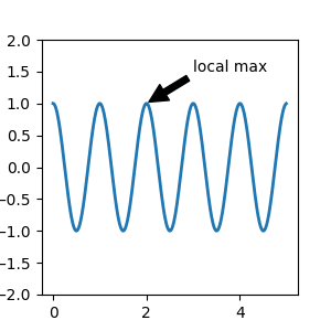
在此示例中,xy(箭头尖端)和 xytext 位置(文本位置)都位于数据坐标中.可以选择多种其他坐标系 -- 你可以使用以下字符串之一为 xycoords 和 textcoords 指定 xy 和 xytext 的坐标系(默认为 'data')
argument |
coordinate system |
|---|---|
'figure points' |
图形左下角的点 |
'figure pixels' |
图形左下角的像素 |
'figure fraction' |
(0, 0) 是图形的左下角,(1, 1) 是右上角 |
'axes points' |
轴左下角的点 |
'axes pixels' |
轴左下角的像素 |
'axes fraction' |
(0, 0) 是轴的左下角,(1, 1) 是右上角 |
'data' |
使用坐标轴数据坐标系 |
以下字符串对于 textcoords 也是有效的参数
argument |
coordinate system |
|---|---|
'offset points' |
从 xy 值偏移(以磅为单位) |
'offset pixels' |
从 xy 值偏移(以像素为单位) |
对于物理坐标系(磅或像素),原点是图形或坐标轴的左下角.磅是 typographic points ,这意味着它们是一个物理单位,测量值为 1/72 英寸.有关点和像素的更多详细信息,请参见 在物理坐标中绘图 .
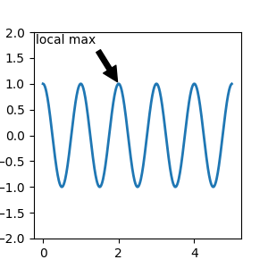
注释数据#
此示例将文本坐标放置在小数值坐标轴坐标中:
fig, ax = plt.subplots(figsize=(3, 3))

t = np.arange(0.0, 5.0, 0.01)
s = np.cos(2*np.pi*t)
line, = ax.plot(t, s, lw=2)

ax.annotate('local max', xy=(2, 1), xycoords='data',
            xytext=(0.01, .99), textcoords='axes fraction',
            va='top', ha='left',
            arrowprops=dict(facecolor='black', shrink=0.05))
ax.set_ylim(-2, 2)
注释一个 Artist#
通过将 Artist 实例作为 xycoords 传入,可以将注释相对于该 Artist 实例定位.然后,xy 将解释为 Artist 边界框的一部分.
import matplotlib.patches as mpatches

fig, ax = plt.subplots(figsize=(3, 3))
arr = mpatches.FancyArrowPatch((1.25, 1.5), (1.75, 1.5),
                               arrowstyle='->,head_width=.15', mutation_scale=20)
ax.add_patch(arr)
ax.annotate("label", (.5, .5), xycoords=arr, ha='center', va='bottom')
ax.set(xlim=(1, 2), ylim=(1, 2))
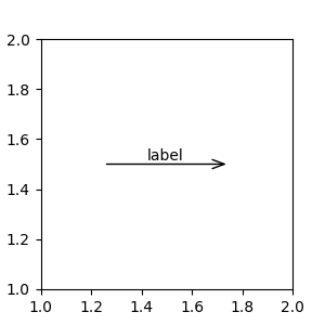
这里,注释放置在相对于箭头左下角的位置 (.5,.5),并且在该位置垂直和水平对齐.垂直方向上,底部与该参考点对齐,以便标签位于线上方.有关链接注释 Artist 的示例,请参见 Artist section 的 注释的坐标系 .
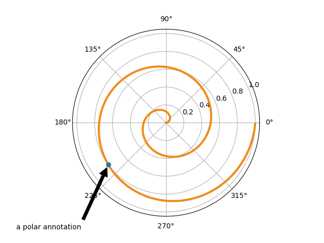
用箭头注释#
您可以通过在可选关键字参数 arrowprops 中提供箭头属性字典来启用从文本到注释点的箭头的绘制.
arrowprops 键 |
描述 |
|---|---|
width |
箭头的宽度(以磅为单位) |
frac |
箭头长度中被箭头头部占据的比例 |
headwidth |
箭头头部底座的宽度(以磅为单位) |
shrink |
将箭头尖端和底座从注释点和文本处移动一定百分比 |
\kwargs |
|
在下面的示例中,由于 xycoords 默认为 'data',因此 xy 点位于数据坐标系中.对于极坐标轴,这是在 (theta, radius) 空间中.此示例中的文本放置在小数值图形坐标系中.像 horizontalalignment,verticalalignment 和 fontsize 这样的 matplotlib.text.Text 关键字参数从 annotate 传递到 Text 实例.
fig = plt.figure()
ax = fig.add_subplot(projection='polar')
r = np.arange(0, 1, 0.001)
theta = 2 * 2*np.pi * r
line, = ax.plot(theta, r, color='#ee8d18', lw=3)

ind = 800
thisr, thistheta = r[ind], theta[ind]
ax.plot([thistheta], [thisr], 'o')
ax.annotate('a polar annotation',
            xy=(thistheta, thisr),  # theta, radius
            xytext=(0.05, 0.05),    # fraction, fraction
            textcoords='figure fraction',
            arrowprops=dict(facecolor='black', shrink=0.05),
            horizontalalignment='left',
            verticalalignment='bottom')
有关绘制箭头的更多信息,请参见 自定义注释箭头
将文本注释相对于数据放置#
通过将 textcoords 关键字参数设置为 'offset points' 或 'offset pixels' ,可以将注释放置在相对于注释的 xy 输入的相对偏移处.
fig, ax = plt.subplots(figsize=(3, 3))
x = [1, 3, 5, 7, 9]
y = [2, 4, 6, 8, 10]
annotations = ["A", "B", "C", "D", "E"]
ax.scatter(x, y, s=20)

for xi, yi, text in zip(x, y, annotations):
    ax.annotate(text,
                xy=(xi, yi), xycoords='data',
                xytext=(1.5, 1.5), textcoords='offset points')
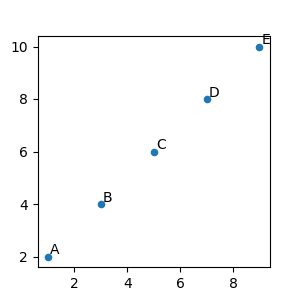
注释从 xy 值偏移 1.5 磅(1.51/72 英寸).
高级注释#
在阅读本节之前,我们建议阅读 Basic annotation , text() 和 annotate() .
使用带框文本进行注释#
text 接受 bbox 关键字参数,该参数在文本周围绘制一个框:
fig, ax = plt.subplots(figsize=(5, 5))
t = ax.text(0.5, 0.5, "Direction",
            ha="center", va="center", rotation=45, size=15,
            bbox=dict(boxstyle="rarrow,pad=0.3",
                      fc="lightblue", ec="steelblue", lw=2))
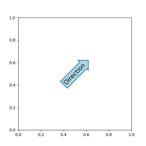
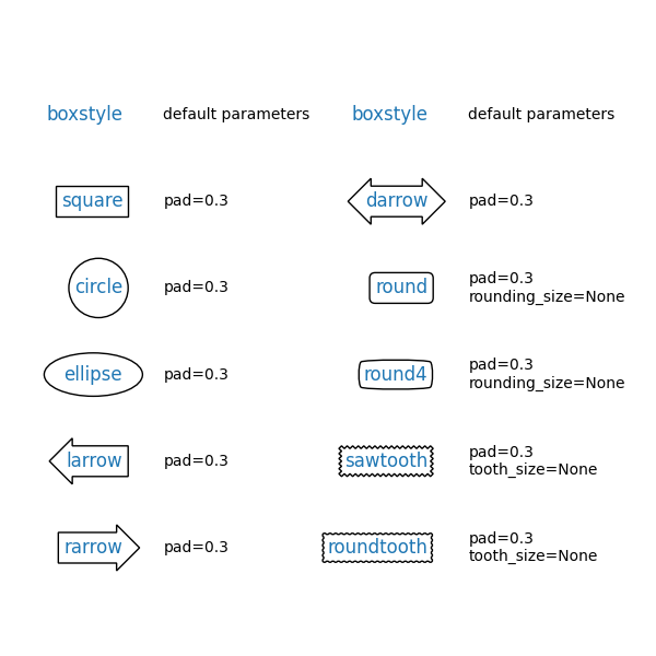
参数是带有其属性作为关键字参数的框样式名称.当前,实现了以下框样式:
类 |
名称 |
属性 |
|---|---|---|
Circle |
|
pad=0.3 |
DArrow |
|
pad=0.3 |
Ellipse |
|
pad=0.3 |
LArrow |
|
pad=0.3 |
RArrow |
|
pad=0.3 |
Round |
|
pad=0.3,rounding_size=None |
Round4 |
|
pad=0.3,rounding_size=None |
Roundtooth |
|
pad=0.3,tooth_size=None |
Sawtooth |
|
pad=0.3,tooth_size=None |
Square |
|
pad=0.3 |
可以使用以下方式访问与文本关联的 patch 对象(框):
bb = t.get_bbox_patch()
返回值是一个 FancyBboxPatch ;可以像往常一样访问和修改 patch 属性(facecolor,edgewidth 等). FancyBboxPatch.set_boxstyle 设置框的形状:
bb.set_boxstyle("rarrow", pad=0.6)
属性参数也可以在使用逗号分隔的样式名称中指定:
bb.set_boxstyle("rarrow, pad=0.6")
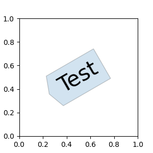
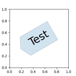
定义自定义框样式#
自定义框样式可以实现为一个函数,该函数接受指定矩形框和"突变"量的参数,并返回"突变"后的路径.具体签名如下面的 custom_box_style 所示.
在这里,我们返回一个新的路径,该路径在框的左侧添加一个"箭头"形状.
然后,可以通过将 bbox=dict(boxstyle=custom_box_style, ...) 传递给 Axes.text 来使用自定义框样式.
from matplotlib.path import Path


def custom_box_style(x0, y0, width, height, mutation_size):
    """
    Given the location and size of the box, return the path of the box around it.

    Rotation is automatically taken care of.

    Parameters
    ----------
    x0, y0, width, height : float
       Box location and size.
    mutation_size : float
        Mutation reference scale, typically the text font size.
    """
    # padding
    mypad = 0.3
    pad = mutation_size * mypad
    # width and height with padding added.
    width = width + 2 * pad
    height = height + 2 * pad
    # boundary of the padded box
    x0, y0 = x0 - pad, y0 - pad
    x1, y1 = x0 + width, y0 + height
    # return the new path
    return Path([(x0, y0), (x1, y0), (x1, y1), (x0, y1),
                 (x0-pad, (y0+y1)/2), (x0, y0), (x0, y0)],
                closed=True)

fig, ax = plt.subplots(figsize=(3, 3))
ax.text(0.5, 0.5, "Test", size=30, va="center", ha="center", rotation=30,
        bbox=dict(boxstyle=custom_box_style, alpha=0.2))
同样,自定义框样式可以实现为实现 __call__ 的类.
然后可以将这些类注册到 BoxStyle._style_list 字典中,这允许将框样式指定为字符串, bbox=dict(boxstyle="registered_name,param=value,...", ...) .请注意,此注册依赖于内部 API,因此未获得官方支持.
from matplotlib.patches import BoxStyle


class MyStyle:
    """A simple box."""

    def __init__(self, pad=0.3):
        """
        The arguments must be floats and have default values.

        Parameters
        ----------
        pad : float
            amount of padding
        """
        self.pad = pad
        super().__init__()

    def __call__(self, x0, y0, width, height, mutation_size):
        """
        Given the location and size of the box, return the path of the box around it.

        Rotation is automatically taken care of.

        Parameters
        ----------
        x0, y0, width, height : float
            Box location and size.
        mutation_size : float
            Reference scale for the mutation, typically the text font size.
        """
        # padding
        pad = mutation_size * self.pad
        # width and height with padding added
        width = width + 2 * pad
        height = height + 2 * pad
        # boundary of the padded box
        x0, y0 = x0 - pad, y0 - pad
        x1, y1 = x0 + width, y0 + height
        # return the new path
        return Path([(x0, y0), (x1, y0), (x1, y1), (x0, y1),
                     (x0-pad, (y0+y1)/2), (x0, y0), (x0, y0)],
                    closed=True)


BoxStyle._style_list["angled"] = MyStyle  # Register the custom style.

fig, ax = plt.subplots(figsize=(3, 3))
ax.text(0.5, 0.5, "Test", size=30, va="center", ha="center", rotation=30,
        bbox=dict(boxstyle="angled,pad=0.5", alpha=0.2))

del BoxStyle._style_list["angled"]  # Unregister it.
类似地,您可以定义自定义的 ConnectionStyle 和自定义的 ArrowStyle .查看 patches 中的源代码,了解每个类的定义方式.
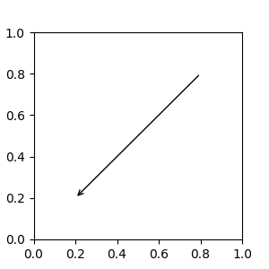
自定义注释箭头#
可以通过指定 arrowprops 参数来选择性地绘制一个连接 xy 和 xytext 的箭头.要仅绘制一个箭头,请使用空字符串作为第一个参数:
fig, ax = plt.subplots(figsize=(3, 3))
ax.annotate("",
            xy=(0.2, 0.2), xycoords='data',
            xytext=(0.8, 0.8), textcoords='data',
            arrowprops=dict(arrowstyle="->", connectionstyle="arc3"))
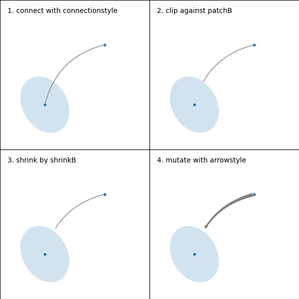
箭头的绘制方式如下:
创建一个连接两点的路径,如 connectionstyle 参数所指定.
如果设置了 patchA 和 patchB,则路径会被裁剪以避开这些补丁.
路径会被 shrinkA 和 shrinkB 进一步缩小(以像素为单位).
路径会按照 arrowstyle 参数的指定转换为箭头补丁.
(png)

两点之间连接路径的创建由 connectionstyle 键控制,以下样式可用:
名称 |
属性 |
|---|---|
|
angleA=90,angleB=0,rad=0.0 |
|
angleA=90,angleB=0 |
|
angleA=0,angleB=0,armA=None,armB=None,rad=0.0 |
|
rad=0.0 |
|
armA=0.0,armB=0.0,fraction=0.3,angle=None |
请注意, angle3 和 arc3 中的"3"表示结果路径是二次样条线段(三个控制点).如下文将要讨论的,一些箭头样式选项只能在连接路径是二次样条线时使用.
以下示例(有限地)演示了每种连接样式的行为.(警告: bar 样式的行为目前未明确定义,将来可能会更改).
(Source code, png)
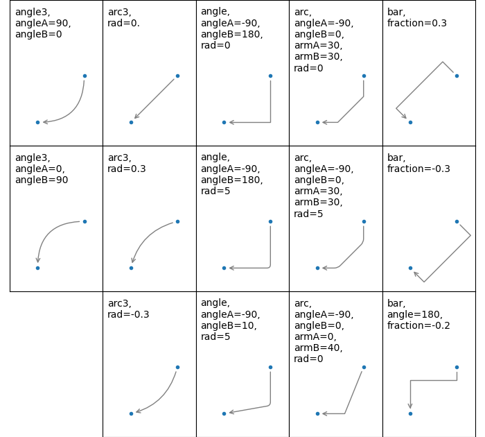
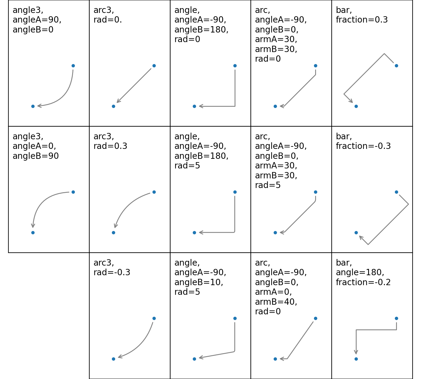
Connection styles for annotations
然后,根据给定的 arrowstyle ,将连接路径(在裁剪和缩小之后)转换为箭头补丁:
名称 |
属性 |
|---|---|
|
None |
|
head_length=0.4,head_width=0.2 |
|
widthB=1.0,lengthB=0.2,angleB=None |
|
widthA=1.0,widthB=1.0 |
|
head_length=0.4,head_width=0.2 |
|
head_length=0.4,head_width=0.2 |
|
head_length=0.4,head_width=0.2 |
|
head_length=0.4,head_width=0.2 |
|
head_length=0.4,head_width=0.2 |
|
head_length=0.4,head_width=0.4,tail_width=0.4 |
|
head_length=0.5,head_width=0.5,tail_width=0.2 |
|
tail_width=0.3,shrink_factor=0.5 |
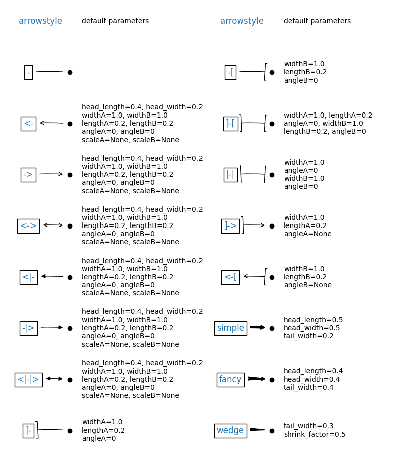
一些箭头样式仅适用于生成二次样条线段的连接样式.它们是 fancy , simple 和 wedge .对于这些箭头样式,您必须使用 "angle3" 或 "arc3" 连接样式.
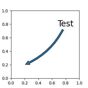
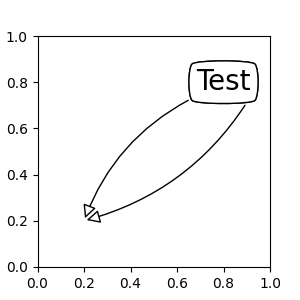
如果给定了annotation string,则默认情况下将补丁设置为文本的bbox patch.
fig, ax = plt.subplots(figsize=(3, 3))

ax.annotate("Test",
            xy=(0.2, 0.2), xycoords='data',
            xytext=(0.8, 0.8), textcoords='data',
            size=20, va="center", ha="center",
            arrowprops=dict(arrowstyle="simple",
                            connectionstyle="arc3,rad=-0.2"))
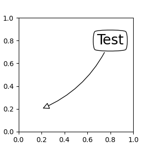
与 text 一样,可以使用 bbox 参数绘制文本周围的框.
fig, ax = plt.subplots(figsize=(3, 3))

ann = ax.annotate("Test",
                  xy=(0.2, 0.2), xycoords='data',
                  xytext=(0.8, 0.8), textcoords='data',
                  size=20, va="center", ha="center",
                  bbox=dict(boxstyle="round4", fc="w"),
                  arrowprops=dict(arrowstyle="-|>",
                                  connectionstyle="arc3,rad=-0.2",
                                  fc="w"))
默认情况下,起点设置为文本范围的中心.可以使用 relpos 键值进行调整.这些值已归一化到文本的范围.例如,(0, 0) 表示左下角,(1, 1) 表示右上角.
fig, ax = plt.subplots(figsize=(3, 3))

ann = ax.annotate("Test",
                  xy=(0.2, 0.2), xycoords='data',
                  xytext=(0.8, 0.8), textcoords='data',
                  size=20, va="center", ha="center",
                  bbox=dict(boxstyle="round4", fc="w"),
                  arrowprops=dict(arrowstyle="-|>",
                                  connectionstyle="arc3,rad=0.2",
                                  relpos=(0., 0.),
                                  fc="w"))

ann = ax.annotate("Test",
                  xy=(0.2, 0.2), xycoords='data',
                  xytext=(0.8, 0.8), textcoords='data',
                  size=20, va="center", ha="center",
                  bbox=dict(boxstyle="round4", fc="w"),
                  arrowprops=dict(arrowstyle="-|>",
                                  connectionstyle="arc3,rad=-0.2",
                                  relpos=(1., 0.),
                                  fc="w"))
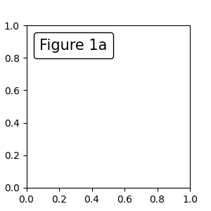
将艺术家放置在锚定的Axes位置#
有一些艺术家类可以放置在 Axes 中的一个锚定位置.一个常见的例子是图例.这种类型的艺术家可以使用 OffsetBox 类来创建. matplotlib.offsetbox 和 mpl_toolkits.axes_grid1.anchored_artists 中提供了一些预定义的类.
from matplotlib.offsetbox import AnchoredText

fig, ax = plt.subplots(figsize=(3, 3))
at = AnchoredText("Figure 1a",
                  prop=dict(size=15), frameon=True, loc='upper left')
at.patch.set_boxstyle("round,pad=0.,rounding_size=0.2")
ax.add_artist(at)
loc 关键字的含义与 legend 命令中相同.
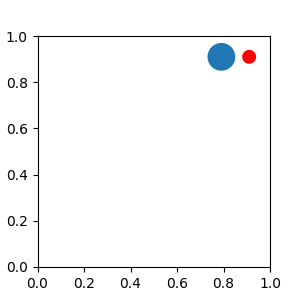
一个简单的应用是在创建时知道艺术家(或艺术家集合)的大小(以像素为单位).例如,如果您想绘制一个固定大小为 20 像素 x 20 像素(半径 = 10 像素)的圆,您可以利用 AnchoredDrawingArea .该实例使用绘图区域的大小(以像素为单位)创建,并且可以将任意艺术家添加到绘图区域.请注意,添加到绘图区域的艺术家的范围与绘图区域本身的位置无关.只有初始大小有关系.
添加到绘图区域的艺术家不应设置变换(它将被覆盖),并且这些艺术家的尺寸被解释为像素坐标,即,以上示例中圆的半径分别为 10 像素和 5 像素.
from matplotlib.patches import Circle
from mpl_toolkits.axes_grid1.anchored_artists import AnchoredDrawingArea

fig, ax = plt.subplots(figsize=(3, 3))
ada = AnchoredDrawingArea(40, 20, 0, 0,
                          loc='upper right', pad=0., frameon=False)
p1 = Circle((10, 10), 10)
ada.drawing_area.add_artist(p1)
p2 = Circle((30, 10), 5, fc="r")
ada.drawing_area.add_artist(p2)
ax.add_artist(ada)
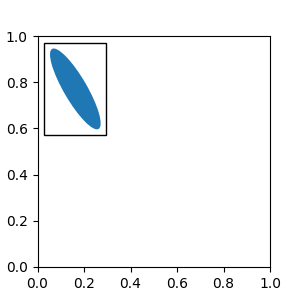
有时,您希望您的艺术家随数据坐标(或画布像素以外的坐标)进行缩放.您可以使用 AnchoredAuxTransformBox 类.这与 AnchoredDrawingArea 类似,不同之处在于,艺术家的大小是在绘制时,根据指定的变换确定的.
下面示例中的椭圆的宽度和高度将分别对应于数据坐标中的 0.1 和 0.4,并且当 Axes 的视图限制更改时,将自动缩放.
from matplotlib.patches import Ellipse
from mpl_toolkits.axes_grid1.anchored_artists import AnchoredAuxTransformBox

fig, ax = plt.subplots(figsize=(3, 3))
box = AnchoredAuxTransformBox(ax.transData, loc='upper left')
el = Ellipse((0, 0), width=0.1, height=0.4, angle=30)  # in data coordinates!
box.drawing_area.add_artist(el)
ax.add_artist(box)
另一种相对于父 Axes 或锚点定位艺术家的的方法是通过 AnchoredOffsetbox 的 bbox_to_anchor 参数.然后可以使用 HPacker 和 VPacker 将此艺术家自动定位到另一个艺术家:
from matplotlib.offsetbox import (AnchoredOffsetbox, DrawingArea, HPacker,
                                  TextArea)

fig, ax = plt.subplots(figsize=(3, 3))

box1 = TextArea(" Test: ", textprops=dict(color="k"))
box2 = DrawingArea(60, 20, 0, 0)

el1 = Ellipse((10, 10), width=16, height=5, angle=30, fc="r")
el2 = Ellipse((30, 10), width=16, height=5, angle=170, fc="g")
el3 = Ellipse((50, 10), width=16, height=5, angle=230, fc="b")
box2.add_artist(el1)
box2.add_artist(el2)
box2.add_artist(el3)

box = HPacker(children=[box1, box2],
              align="center",
              pad=0, sep=5)

anchored_box = AnchoredOffsetbox(loc='lower left',
                                 child=box, pad=0.,
                                 frameon=True,
                                 bbox_to_anchor=(0., 1.02),
                                 bbox_transform=ax.transAxes,
                                 borderpad=0.,)

ax.add_artist(anchored_box)
fig.subplots_adjust(top=0.8)
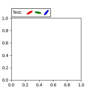
请注意,与 Legend 中不同, bbox_transform 默认设置为 IdentityTransform
注释的坐标系#
Matplotlib Annotations 支持多种坐标系. Basic annotation 中的示例使用了 data 坐标系; 一些更高级的选项是:
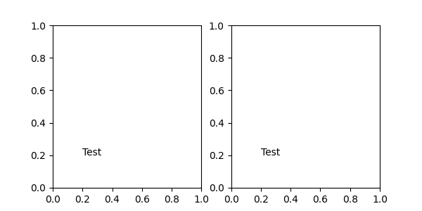
Transform 实例#
Transforms 将坐标映射到不同的坐标系中,通常是显示坐标系.有关详细说明,请参见 转换教程 .在这里,Transform 对象用于标识相应点的坐标系.例如, Axes.transAxes 变换将注释相对于 Axes 坐标进行定位;因此,使用它与将坐标系设置为"axes fraction"相同:
fig, (ax1, ax2) = plt.subplots(nrows=1, ncols=2, figsize=(6, 3))
ax1.annotate("Test", xy=(0.2, 0.2), xycoords=ax1.transAxes)
ax2.annotate("Test", xy=(0.2, 0.2), xycoords="axes fraction")
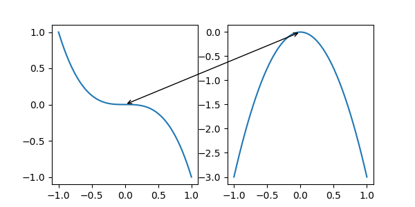
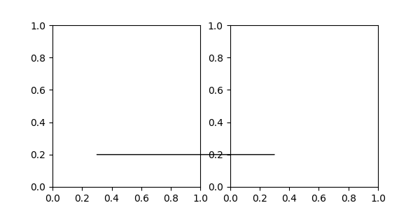
另一个常用的 Transform 实例是 Axes.transData .此变换是 Axes 中绘制的数据的坐标系.在此示例中,它用于在两个 Axes 中绘制相关数据点之间的箭头.我们传递了一个空文本,因为在这种情况下,注释连接了数据点.
x = np.linspace(-1, 1)

fig, (ax1, ax2) = plt.subplots(nrows=1, ncols=2, figsize=(6, 3))
ax1.plot(x, -x**3)
ax2.plot(x, -3*x**2)
ax2.annotate("",
             xy=(0, 0), xycoords=ax1.transData,
             xytext=(0, 0), textcoords=ax2.transData,
             arrowprops=dict(arrowstyle="<->"))
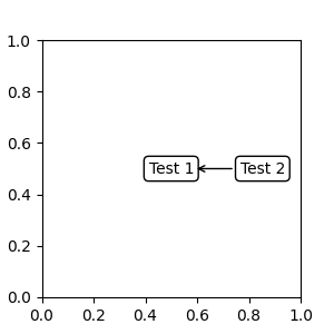
Artist 实例#
xy 值(或 xytext)被解释为艺术家边界框 (bbox) 的分数坐标:
fig, ax = plt.subplots(nrows=1, ncols=1, figsize=(3, 3))
an1 = ax.annotate("Test 1",
                  xy=(0.5, 0.5), xycoords="data",
                  va="center", ha="center",
                  bbox=dict(boxstyle="round", fc="w"))

an2 = ax.annotate("Test 2",
                  xy=(1, 0.5), xycoords=an1,  # (1, 0.5) of an1's bbox
                  xytext=(30, 0), textcoords="offset points",
                  va="center", ha="left",
                  bbox=dict(boxstyle="round", fc="w"),
                  arrowprops=dict(arrowstyle="->"))

请注意,您必须确保在绘制 an2 之前确定坐标艺术家(在此示例中为 an1)的范围.通常,这意味着 an2 需要在 an1 之后绘制.所有边界框的基类是 BboxBase
返回 Transform of BboxBase 的可调用对象#
一个可调用对象,它将渲染器实例作为单个参数,并返回 Transform 或 BboxBase .例如, Artist.get_window_extent 的返回值是一个 bbox,因此此方法与 (2) 传入 artist 相同:
fig, ax = plt.subplots(nrows=1, ncols=1, figsize=(3, 3))
an1 = ax.annotate("Test 1",
                  xy=(0.5, 0.5), xycoords="data",
                  va="center", ha="center",
                  bbox=dict(boxstyle="round", fc="w"))

an2 = ax.annotate("Test 2",
                  xy=(1, 0.5), xycoords=an1.get_window_extent,
                  xytext=(30, 0), textcoords="offset points",
                  va="center", ha="left",
                  bbox=dict(boxstyle="round", fc="w"),
                  arrowprops=dict(arrowstyle="->"))
Artist.get_window_extent 是 Axes 对象的边界框,因此与将坐标系设置为 axes fraction 相同:
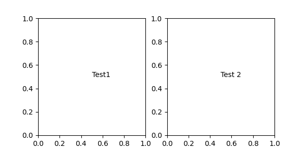
fig, (ax1, ax2) = plt.subplots(nrows=1, ncols=2, figsize=(6, 3))

an1 = ax1.annotate("Test1", xy=(0.5, 0.5), xycoords="axes fraction")
an2 = ax2.annotate("Test 2", xy=(0.5, 0.5), xycoords=ax2.get_window_extent)
混合坐标规范#
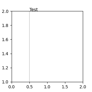
一对混合的坐标规范--第一个用于 x 坐标,第二个用于 y 坐标.例如,x=0.5 采用数据坐标,y=1 采用归一化 axes 坐标:
fig, ax = plt.subplots(figsize=(3, 3))
ax.annotate("Test", xy=(0.5, 1), xycoords=("data", "axes fraction"))
ax.axvline(x=.5, color='lightgray')
ax.set(xlim=(0, 2), ylim=(1, 2))
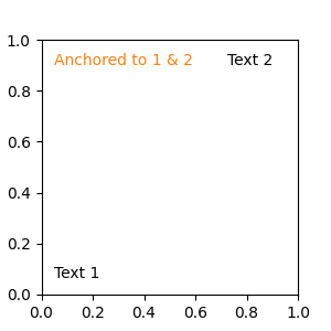
任何受支持的坐标系都可以在混合规范中使用.例如,文本"Anchored to 1 & 2"相对于两个 Text 艺术家定位:
fig, ax = plt.subplots(figsize=(3, 3))

t1 = ax.text(0.05, .05, "Text 1", va='bottom', ha='left')
t2 = ax.text(0.90, .90, "Text 2", ha='right')
t3 = ax.annotate("Anchored to 1 & 2", xy=(0, 0), xycoords=(t1, t2),
                 va='bottom', color='tab:orange',)
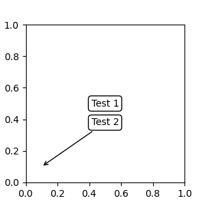
text.OffsetFrom#
有时,您希望您的注释具有一些"偏移点",而不是来自注释点,而是来自其他点或艺术家. text.OffsetFrom 是这种情况的助手.
from matplotlib.text import OffsetFrom

fig, ax = plt.subplots(figsize=(3, 3))
an1 = ax.annotate("Test 1", xy=(0.5, 0.5), xycoords="data",
                  va="center", ha="center",
                  bbox=dict(boxstyle="round", fc="w"))

offset_from = OffsetFrom(an1, (0.5, 0))
an2 = ax.annotate("Test 2", xy=(0.1, 0.1), xycoords="data",
                  xytext=(0, -10), textcoords=offset_from,
                  # xytext is offset points from "xy=(0.5, 0), xycoords=an1"
                  va="top", ha="center",
                  bbox=dict(boxstyle="round", fc="w"),
                  arrowprops=dict(arrowstyle="->"))
非文本注释#
使用 ConnectionPatch#
ConnectionPatch 就像一个没有文本的注释.虽然 annotate 在大多数情况下都足够了,但是当您想连接不同 Axes 中的点时, ConnectionPatch 会很有用.例如,这里我们将 ax1 的数据坐标中的点 xy 连接到 ax2 的数据坐标中的点 xy:
from matplotlib.patches import ConnectionPatch

fig, (ax1, ax2) = plt.subplots(nrows=1, ncols=2, figsize=(6, 3))
xy = (0.3, 0.2)
con = ConnectionPatch(xyA=xy, coordsA=ax1.transData,
                      xyB=xy, coordsB=ax2.transData)

fig.add_artist(con)
在这里,我们将 ConnectionPatch 添加到图形(使用 add_artist )而不是添加到任何一个 Axes.这确保了 ConnectionPatch 艺术家绘制在两个 Axes 的顶部,并且在使用 constrained_layout 定位 Axes 时也是必需的.
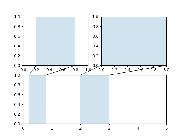
Axes 之间的缩放效果#
mpl_toolkits.axes_grid1.inset_locator 定义了一些用于连接两个 Axes 的 patch 类.
脚本的总运行时间:(0 分 4.143 秒)