Tight layout guide

How to use tight-layout to fit plots within your figure cleanly.

tight_layout 自动调整子图参数,使子图适合图形区域.这是一个实验性功能,可能不适用于某些情况.它只检查刻度标签,轴标签和标题的范围.

An alternative to tight_layout is constrained_layout .

简单示例

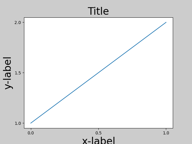
使用默认的 Axes 定位,坐标轴标题,轴标签或刻度标签有时会超出图形区域,因此会被裁剪.

import matplotlib.pyplot as plt
import numpy as np

plt.rcParams['savefig.facecolor'] = "0.8"


def example_plot(ax, fontsize=12):
    ax.plot([1, 2])

    ax.locator_params(nbins=3)
    ax.set_xlabel('x-label', fontsize=fontsize)
    ax.set_ylabel('y-label', fontsize=fontsize)
    ax.set_title('Title', fontsize=fontsize)

plt.close('all')
fig, ax = plt.subplots()
example_plot(ax, fontsize=24)

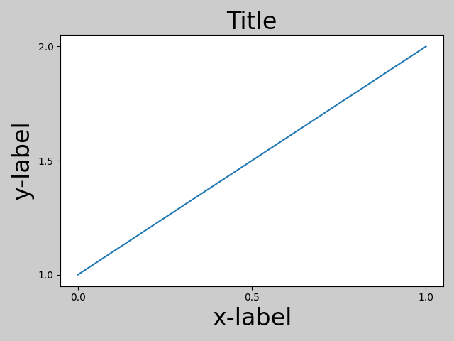
为了防止这种情况,需要调整Axes的位置.对于子图,可以通过使用 Figure.subplots_adjust 调整子图参数来手动完成. Figure.tight_layout 会自动执行此操作.

fig, ax = plt.subplots()
example_plot(ax, fontsize=24)
plt.tight_layout()

请注意, matplotlib.pyplot.tight_layout() 仅在调用时调整子图参数.为了在每次重绘图形时执行此调整,您可以调用 fig.set_tight_layout(True) ,或者等效地,将 rcParams["figure.autolayout"] (default: False) 设置为 True .

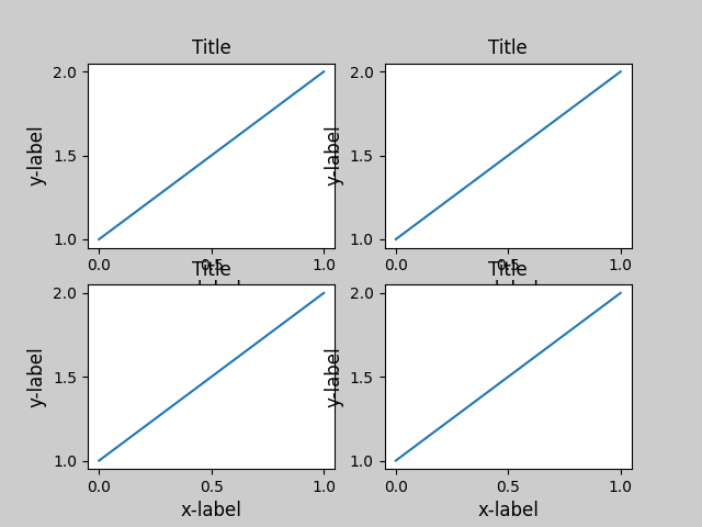
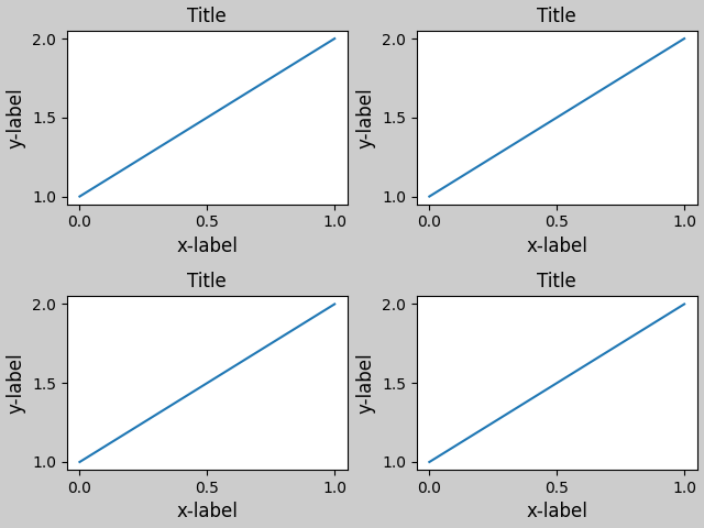
当您有多个子图时,通常会看到不同 Axes 的标签相互重叠.

plt.close('all')

fig, ((ax1, ax2), (ax3, ax4)) = plt.subplots(nrows=2, ncols=2)
example_plot(ax1)
example_plot(ax2)
example_plot(ax3)
example_plot(ax4)

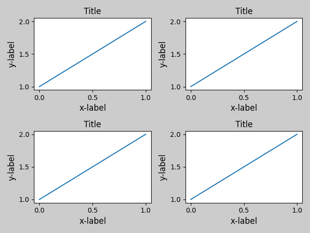
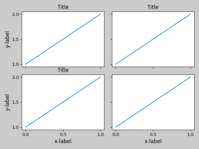
tight_layout() 也会调整子图之间的间距,以最大限度地减少重叠.

fig, ((ax1, ax2), (ax3, ax4)) = plt.subplots(nrows=2, ncols=2)
example_plot(ax1)
example_plot(ax2)
example_plot(ax3)
example_plot(ax4)
plt.tight_layout()

tight_layout() 可以接受 pad,w_pad 和 h_pad 的关键字参数.这些参数控制图形边框周围和子图之间的额外填充.填充以字体大小的分数指定.

fig, ((ax1, ax2), (ax3, ax4)) = plt.subplots(nrows=2, ncols=2)
example_plot(ax1)
example_plot(ax2)
example_plot(ax3)
example_plot(ax4)
plt.tight_layout(pad=0.4, w_pad=0.5, h_pad=1.0)

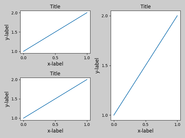
只要它们的网格规范兼容, tight_layout() 即使子图的大小不同也能工作.在下面的示例中,ax1 和 ax2 是 2x2 网格的子图,而 ax3 是 1x2 网格的子图.

plt.close('all')
fig = plt.figure()

ax1 = plt.subplot(221)
ax2 = plt.subplot(223)
ax3 = plt.subplot(122)

example_plot(ax1)
example_plot(ax2)
example_plot(ax3)

plt.tight_layout()

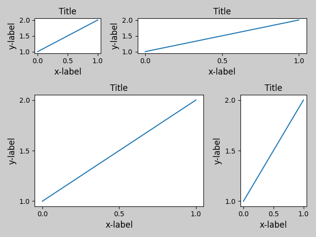
它适用于使用 subplot2grid() 创建的子图.通常,从网格规范 ( 在 Figure 中排列多个 Axes ) 创建的子图将起作用.

plt.close('all')
fig = plt.figure()

ax1 = plt.subplot2grid((3, 3), (0, 0))
ax2 = plt.subplot2grid((3, 3), (0, 1), colspan=2)
ax3 = plt.subplot2grid((3, 3), (1, 0), colspan=2, rowspan=2)
ax4 = plt.subplot2grid((3, 3), (1, 2), rowspan=2)

example_plot(ax1)
example_plot(ax2)
example_plot(ax3)
example_plot(ax4)

plt.tight_layout()

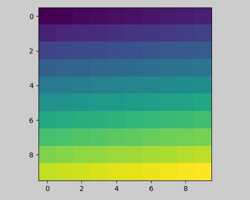
虽然没有经过彻底的测试,但它似乎适用于 aspect != "auto" 的子图(例如,带有图像的 Axes).

arr = np.arange(100).reshape((10, 10))

plt.close('all')
fig = plt.figure(figsize=(5, 4))

ax = plt.subplot()
im = ax.imshow(arr, interpolation="none")

plt.tight_layout()

Caveats

• 默认情况下, tight_layout 会考虑 Axes 上的所有艺术家.要从布局计算中删除艺术家,您可以调用 Artist.set_in_layout .

• tight_layout 假定艺术家所需的额外空间与 Axes 的原始位置无关.这通常是正确的,但在极少数情况下并非如此.

• pad=0 可能会裁剪一些文本几个像素.这可能是当前算法的一个 bug 或一个限制,目前尚不清楚为什么会发生这种情况.同时,建议使用大于 0.3 的 pad.

与 GridSpec 一起使用

GridSpec 有自己的 GridSpec.tight_layout 方法(pyplot api pyplot.tight_layout 也有效).

import matplotlib.gridspec as gridspec

plt.close('all')
fig = plt.figure()

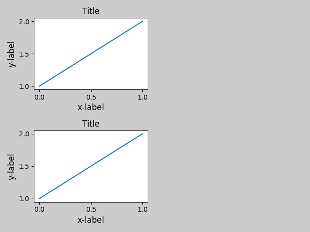
gs1 = gridspec.GridSpec(2, 1)
ax1 = fig.add_subplot(gs1[0])
ax2 = fig.add_subplot(gs1[1])

example_plot(ax1)
example_plot(ax2)

gs1.tight_layout(fig)

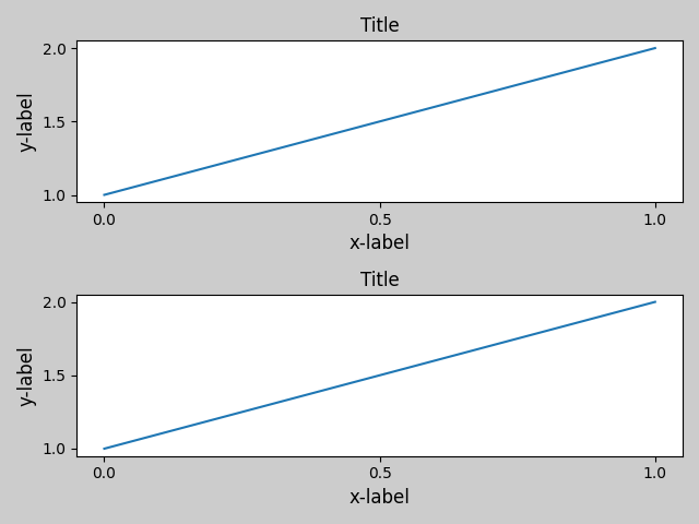
您可以提供一个可选的 rect 参数,该参数指定子图将适合的边界框.坐标采用归一化图形坐标,默认为 (0, 0, 1, 1)(整个图形).

fig = plt.figure()

gs1 = gridspec.GridSpec(2, 1)
ax1 = fig.add_subplot(gs1[0])
ax2 = fig.add_subplot(gs1[1])

example_plot(ax1)
example_plot(ax2)

gs1.tight_layout(fig, rect=[0, 0, 0.5, 1.0])

但是,我们不建议使用它来手动构建更复杂的布局,例如在图形的左侧有一个 GridSpec,在右侧有一个 GridSpec.对于这些用例,应该利用 嵌套的 Gridspecs 或 图形子图 .

Legends and annotations

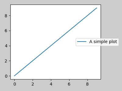
Pre Matplotlib 2.2, legends and annotations were excluded from the bounding box calculations that decide the layout. Subsequently, these artists were added to the calculation, but sometimes it is undesirable to include them. For instance in this case it might be good to have the Axes shrink a bit to make room for the legend:

fig, ax = plt.subplots(figsize=(4, 3))
lines = ax.plot(range(10), label='A simple plot')
ax.legend(bbox_to_anchor=(0.7, 0.5), loc='center left',)
fig.tight_layout()
plt.show()

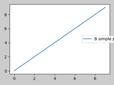
然而,有时这是不需要的(通常在使用 fig.savefig('outname.png', bbox_inches='tight') 时).为了从边界框计算中移除图例,我们只需将其边界 leg.set_in_layout(False) ,图例将被忽略.

fig, ax = plt.subplots(figsize=(4, 3))
lines = ax.plot(range(10), label='B simple plot')
leg = ax.legend(bbox_to_anchor=(0.7, 0.5), loc='center left',)
leg.set_in_layout(False)
fig.tight_layout()
plt.show()

与 AxesGrid1 一起使用

提供了对 mpl_toolkits.axes_grid1 的有限支持.

from mpl_toolkits.axes_grid1 import Grid

plt.close('all')
fig = plt.figure()
grid = Grid(fig, rect=111, nrows_ncols=(2, 2),
            axes_pad=0.25, label_mode='L',
            )

for ax in grid:
    example_plot(ax)
ax.title.set_visible(False)

plt.tight_layout()

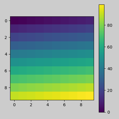
颜色条

如果您使用 Figure.colorbar 创建颜色条,则创建的颜色条将在子图中绘制,只要父 Axes 也是子图,因此 Figure.tight_layout 将起作用.

plt.close('all')
arr = np.arange(100).reshape((10, 10))
fig = plt.figure(figsize=(4, 4))
im = plt.imshow(arr, interpolation="none")

plt.colorbar(im)

plt.tight_layout()

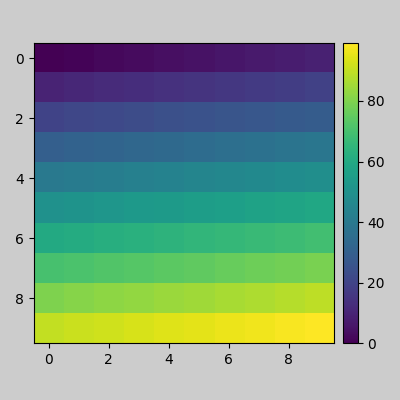
另一种选择是使用 AxesGrid1 工具包显式地为颜色条创建一个 Axes.

from mpl_toolkits.axes_grid1 import make_axes_locatable

plt.close('all')
arr = np.arange(100).reshape((10, 10))
fig = plt.figure(figsize=(4, 4))
im = plt.imshow(arr, interpolation="none")

divider = make_axes_locatable(plt.gca())
cax = divider.append_axes("right", "5%", pad="3%")
plt.colorbar(im, cax=cax)

plt.tight_layout()